---
# Content: CC BY-NC-SA 4.0 | Code: MIT - see /LICENSE.md
title: "Natural language processing for business"
---
{{< include /_common-imports.qmd >}}
## Text is just another data type {#sec-nlp-intro}
You've parsed log files, tokenised configuration strings, validated user input with regular expressions, and built search indices over documentation. Text processing is a core part of software engineering. But there's a fundamental difference between parsing structured text, where the format is known and the grammar is formal, and extracting meaning from *unstructured* text, where the same idea can be expressed in dozens of different ways and the "schema" is the entirety of human language.
Consider a customer support system. A rule-based router can match keywords: if the message contains "billing" or "invoice," send it to the finance team. But what about "I was charged twice for the same thing" or "my card got hit with a payment I don't recognise"? Neither mentions "billing" or "invoice," yet both are billing issues. The vocabulary is enormous, the phrasing is unpredictable, and synonymy (different words, same meaning) and polysemy (same word, different meanings) make simple string matching brittle.
Natural language processing (NLP) applies the statistical and modelling tools from earlier chapters to this problem. Instead of writing rules by hand for every possible phrasing, we represent text numerically, then let classification and clustering algorithms find patterns in the numbers. The representation is the hard part: once text is a matrix, the machinery of logistic regression (@sec-from-numbers-to-decisions), tree models (@sec-decision-trees), and dimensionality reduction (@sec-too-many-features) applies directly.
The goal is to understand the statistical foundations that make text classification work, not to deploy a state-of-the-art system. We build a complete NLP pipeline for a realistic business problem — routing customer support tickets to the correct team — using only the standard scikit-learn stack.
## The data: customer support tickets {#sec-nlp-data}
We'll simulate a dataset of support tickets for a SaaS platform. Each ticket has a text body and a category label representing the team that should handle it. The simulation captures realistic properties: varied phrasing, overlapping vocabulary between categories, and the kind of conversational noise that makes text classification harder than it looks.
```{python}
#| label: nlp-data-setup
#| echo: true
#| code-fold: true
#| code-summary: "Expand to see ticket simulation code"
rng = np.random.default_rng(42)

# --- Vocabulary pools ---
# Each category has a "core" vocabulary (strongly indicative) and a
# "shared" vocabulary (appears across categories).  Tickets are built
# by combining phrases from both pools, which creates realistic
# cross-category overlap — the same reason keyword matching fails.

core_phrases = {
    'billing': [
        'charged twice', 'unexpected charge', 'need a refund',
        'overcharged on my invoice', 'billing discrepancy',
        'auto-renewal charged me', 'receipt for expenses',
        'charged more than the quote', 'payment failed',
        "discount code didn't work", 'credit card was billed',
        'invoice is higher than usual', 'double charge',
        "refund still hasn't arrived", "pricing doesn't match",
    ],
    'technical': [
        '500 error on export', 'API returns a timeout',
        "dashboard won't load", 'getting a loading spinner',
        'search returns no results', 'webhook not receiving events',
        'CSV export missing columns', 'SSO integration broke',
        'mobile app crashes', 'data sync is broken',
        "can't upload files", 'performance has degraded',
        'scheduled reports are blank', 'form throws an error',
    ],
    'account': [
        'add new users to our team', 'transfer account ownership',
        'reset two-factor authentication', 'merge two accounts',
        'update the company name', 'change my email address',
        'set up role-based permissions', 'remove a former employee',
        'forgot my password', 'change the primary admin',
        'audit log of account access', 'enable single sign-on',
        "can't see the shared workspace", 'set up separate workspaces',
    ],
    'feature_request': [
        'would be great to have dark mode', 'schedule reports for delivery',
        'need a Slack integration', 'add bulk editing',
        'want a kanban view', 'custom branding on the login page',
        'support importing from spreadsheets', 'mobile app for iOS',
        'granular notification preferences', 'changelog page',
        'export as PDF not just CSV', 'automated alerts for metrics',
        'hardware key authentication', 'API endpoint for user management',
    ],
}

# Shared vocabulary that can appear in ANY category — these dilute
# the category-specific signal and create realistic ambiguity
shared_openers = [
    'I need help with', 'Can someone look into', 'Quick question about',
    'Following up on', 'Having trouble with', 'Is there a way to',
    "I'd like to", 'We need to', 'Please help with',
    'Our team is struggling with', 'Urgent issue regarding',
    'Could you assist with', 'Not sure who to ask about',
]

shared_context = [
    'my account', 'our team account', 'the enterprise plan',
    'the dashboard', 'the settings page', 'the upgrade we did',
    'the new update', 'our organisation', 'my profile',
    'the notification settings', 'our billing portal',
    'the export feature', 'our integration', 'the API',
    'the login page', 'the admin panel',
]

shared_closings = [
    'This is affecting our whole team.',
    "I've been a customer for two years.",
    'This is urgent for our quarterly deadline.',
    "I've already tried the troubleshooting guide.",
    'Other people on my team have the same issue.',
    'Please escalate this if needed.',
    'Is there a workaround in the meantime?',
    'Happy to jump on a call to discuss.',
    'I contacted support before about this.',
    'We really like the product but this is frustrating.',
    'Thanks in advance for your help.',
    'Appreciate any guidance on this.',
]

# Categories that share vocabulary and get confused by classifiers
confusion_neighbours = {
    'billing': ['account'],
    'technical': ['feature_request'],
    'account': ['billing', 'technical'],
    'feature_request': ['technical'],
}

rows = []
for category, phrases in core_phrases.items():
    n_tickets = rng.integers(200, 280)
    for _ in range(n_tickets):
        parts = []

        # 30% chance: start with a shared opener (dilutes signal)
        if rng.random() < 0.30:
            parts.append(rng.choice(shared_openers))

        # Core phrase — the main category signal.
        # 12% of the time, use a phrase from a neighbouring category.
        # This simulates real tickets where a customer writes about
        # their billing issue using account language, or reports a
        # bug that reads like a feature request.
        if rng.random() < 0.12:
            neighbour = rng.choice(confusion_neighbours[category])
            parts.append(rng.choice(core_phrases[neighbour]))
        else:
            parts.append(rng.choice(phrases))

        # 25% chance: add shared context (creates cross-category overlap)
        if rng.random() < 0.25:
            parts.append('on ' + rng.choice(shared_context))

        # 30% chance: append a shared closing sentence
        if rng.random() < 0.30:
            parts.append(rng.choice(shared_closings))

        text = ' '.join(parts)

        # 15% chance: randomly drop 1-2 words (simulates casual text)
        if rng.random() < 0.15:
            words = text.split()
            if len(words) > 6:
                for _ in range(rng.integers(1, 3)):
                    idx = rng.integers(1, len(words) - 1)
                    words.pop(idx)
                text = ' '.join(words)

        rows.append({'text': text, 'category': category})

tickets = pd.DataFrame(rows)
tickets = tickets.sample(frac=1, random_state=42).reset_index(drop=True)

print(f"Total tickets: {len(tickets):,}")
print(f"\nCategory distribution:")
print(tickets['category'].value_counts().to_string())
print(f"\nExample tickets:")
for cat in core_phrases:
    example = tickets[tickets['category'] == cat].iloc[0]
    print(f"  [{cat:16s}] {example['text'][:80]}...")
```
The category distribution is roughly balanced; each team handles a similar volume. In practice, categories are often heavily skewed (billing issues might be 50% of all tickets while feature requests are 5%), which would bring back the class imbalance challenges from @sec-fraud-imbalance. We'll keep the distribution balanced here to focus on the text representation problem.
::: {.callout-note}
## Engineering Bridge
If you've built a log classification system, routing log lines to different handlers based on content, this is structurally the same problem. The difference is that log lines follow a semi-structured format (timestamp, severity, service name, message), while support tickets are free-form natural language. Log classification can often be solved with regular expressions and pattern matching because the vocabulary is constrained by your application's logging framework. Support ticket classification can't, because the vocabulary is constrained only by the English language and your customers' creativity.
:::
## From text to numbers: the representation problem {#sec-nlp-representation}
Machine learning algorithms operate on numbers, not strings. The core challenge in NLP is **representation** — converting variable-length text into fixed-length numerical vectors that preserve the meaning well enough for a classifier to work with.
The simplest approach is the **bag of words** (BoW) model. Treat each unique word in the corpus as a feature dimension. For each document, count how many times each word appears. The result is a matrix where rows are documents and columns are words: a high-dimensional, sparse representation that ignores word order entirely.
```{python}
#| label: nlp-bow-example
#| echo: true
from sklearn.feature_extraction.text import CountVectorizer

# A small example to show what BoW produces
example_texts = [
    'The dashboard keeps crashing',
    'My invoice has the wrong amount',
    'The dashboard shows the wrong data',
]

bow = CountVectorizer()
X_example = bow.fit_transform(example_texts)

bow_df = pd.DataFrame(
    X_example.toarray(),
    columns=bow.get_feature_names_out(),
    index=[f"doc_{i}" for i in range(len(example_texts))]
)
print(bow_df.to_string())
```
Documents 0 and 2 share "the" and "dashboard"; the model can detect that overlap. But "the" appears in every document and tells us nothing about category. "Dashboard" is genuinely informative (it suggests a technical issue), while "the" is noise. We need a way to down-weight common words and up-weight distinctive ones.
**TF-IDF** (term frequency–inverse document frequency) does exactly this. For each word $t$ in document $d$:
$$
\text{tf-idf}(t, d) = \text{tf}(t, d) \times \log\frac{N}{\text{df}(t)}
$$
where $\text{tf}(t, d)$ is how often word $t$ appears in document $d$, $N$ is the total number of documents, and $\text{df}(t)$ is how many documents contain $t$. Words that appear in many documents get a low IDF (inverse document frequency) and are down-weighted. Words that appear in few documents get a high IDF and are amplified. The logarithm prevents rare words from being weighted *too* aggressively. (Scikit-learn's implementation adds smoothing, $\log\frac{1 + N}{1 + \text{df}(t)} + 1$, and then L2-normalises each row, so the raw formula above is the intuition rather than the exact computation.)
```{python}
#| label: nlp-tfidf-example
#| echo: true
from sklearn.feature_extraction.text import TfidfVectorizer

tfidf = TfidfVectorizer()
X_tfidf_example = tfidf.fit_transform(example_texts)

tfidf_df = pd.DataFrame(
    X_tfidf_example.toarray().round(3),
    columns=tfidf.get_feature_names_out(),
    index=[f"doc_{i}" for i in range(len(example_texts))]
)
print(tfidf_df.to_string())
```
Notice how "the" now has a lower weight relative to "dashboard," "invoice," and "crashing." The TF-IDF representation captures which words are *distinctive* to each document, not just which words are *present*.
::: {.callout-tip}
## Author's Note
The bag-of-words representation felt profoundly wrong at first. Throwing away word order means "the dog bit the man" and "the man bit the dog" get identical representations. My instinct as an engineer was that this information loss would be fatal: how can you understand meaning without understanding structure? But in practice, for many business classification tasks, the bag of words is *enough*. The category of a support ticket depends far more on *which words* appear (dashboard, invoice, upgrade, integration) than on their order. This is a useful lesson in pragmatism: a lossy representation that captures the right information can outperform a richer representation that captures everything but diffuses the signal.
:::
## Preprocessing: what to keep and what to discard {#sec-nlp-preprocessing}
Before vectorising, we need to decide how to tokenise the text, how to split it into units. Scikit-learn's vectorisers handle this with sensible defaults (split on whitespace and punctuation, convert to lowercase), but several preprocessing choices have a significant impact on downstream performance.
**Stop word removal** eliminates common function words ("the," "is," "and") that carry little semantic content. **N-grams** extend the vocabulary beyond single words: bigrams like "dark mode" or "credit card" capture phrases that lose meaning when split into individual words. The trade-off is vocabulary size: adding bigrams can increase the feature space by an order of magnitude.
```{python}
#| label: nlp-preprocessing-comparison
#| echo: true
from sklearn.model_selection import cross_val_score
from sklearn.linear_model import LogisticRegression
from sklearn.pipeline import Pipeline
from sklearn.base import clone

configs = {
    'Unigrams only': TfidfVectorizer(),
    'Unigrams + bigrams': TfidfVectorizer(ngram_range=(1, 2)),
    'With stop words removed': TfidfVectorizer(stop_words='english'),
    'Bigrams + stop words': TfidfVectorizer(
        ngram_range=(1, 2), stop_words='english'
    ),
}

y = tickets['category']

print(f"{'Configuration':<30s} {'Vocab size':>12s} {'CV accuracy':>14s}")
print('-' * 58)

for name, vec in configs.items():
    pipe = Pipeline([
        ('tfidf', vec),
        ('clf', LogisticRegression(max_iter=1000, random_state=42)),
    ])
    scores = cross_val_score(pipe, tickets['text'], y, cv=5, scoring='accuracy')
    # Fit a throwaway clone purely to read off vocabulary size, so we
    # don't mutate or refit the vectoriser used inside the pipeline
    vec_fitted = clone(vec).fit(tickets['text'])
    print(f"{name:<30s} {len(vec_fitted.vocabulary_):>12,d} {scores.mean():>11.1%} ± {scores.std():.1%}")
```
For this dataset, the differences between configurations are modest. Stop word removal helps slightly (it removes high-frequency noise words from the TF-IDF representation), while bigrams capture meaningful phrases like "credit card" and "dark mode" but also inflate the vocabulary substantially. This is typical for text classification tasks where the category-specific vocabulary is strong enough that marginal representation improvements don't move the needle dramatically.
We'll use the bigrams-plus-stop-words configuration for the rest of this chapter; it's a good default that balances vocabulary size against representation quality.
## Building the classifier {#sec-nlp-classification}
With text represented as TF-IDF vectors, classification is logistic regression on a very high-dimensional sparse matrix. The linear model's strength here comes from the same mathematical property that makes regularisation work (@sec-ridge): when you have many features (words) but relatively few examples, a model that constrains its complexity by penalising large coefficients generalises better than one that can fit arbitrary boundaries.
```{python}
#| label: nlp-model-setup
#| echo: true
from sklearn.model_selection import train_test_split
from sklearn.metrics import classification_report

X_train_text, X_test_text, y_train, y_test = train_test_split(
    tickets['text'], tickets['category'],
    test_size=0.2, random_state=42, stratify=tickets['category']
)

# Vectorise using training data only — avoid data leakage
vectoriser = TfidfVectorizer(ngram_range=(1, 2), stop_words='english')
X_train = vectoriser.fit_transform(X_train_text)
X_test = vectoriser.transform(X_test_text)

print(f"Training set: {X_train.shape[0]:,} tickets, {X_train.shape[1]:,} features")
print(f"Test set:     {X_test.shape[0]:,} tickets")
print(f"Matrix density: {X_train.nnz / (X_train.shape[0] * X_train.shape[1]):.4%}")
```
The matrix density confirms the extreme sparsity of text data: each document uses only a tiny fraction of the total vocabulary. Now let's fit a logistic regression classifier and examine its performance.
```{python}
#| label: nlp-logistic-regression
#| echo: true
lr = LogisticRegression(max_iter=1000, random_state=42)
lr.fit(X_train, y_train)

y_pred_lr = lr.predict(X_test)

print('Logistic regression — classification report:\n')
print(classification_report(y_test, y_pred_lr))
```
The per-class F1 scores show where the model succeeds and struggles. Categories with distinctive vocabulary (technical issues mentioning "error," "API," "timeout") tend to score higher than categories with vocabulary that overlaps other classes (account tickets mentioning "billing," feature requests mentioning "dashboard"). This asymmetry in difficulty is inherent to the data, not a modelling failure.
Sparsity is also why linear models like logistic regression tend to outperform tree-based models on sparse, high-dimensional text. Gradient boosting splits on individual features, and when most features are zero for most documents, each split carries little information. Logistic regression computes a weighted sum across *all* features simultaneously, and the TF-IDF weighting ensures that the non-zero entries are the informative ones.
::: {.callout-note}
## Engineering Bridge
The sparse TF-IDF matrix is conceptually similar to a **sparse configuration matrix** in distributed systems. Each document "enables" a small subset of features (words) from a large vocabulary, just as each request or user session activates a small subset of paths through your application. The same storage and computation strategies apply: don't materialise the full dense matrix, use sparse representations, and design algorithms that handle sparsity efficiently. Scikit-learn's `TfidfVectorizer` returns `scipy.sparse` matrices specifically for this reason: fitting a model on a dense 800×3,000 matrix is feasible, but the equivalent operation on a dense 100,000×500,000 matrix (a realistic production vocabulary) would exhaust memory.
:::
## Interpreting the classifier {#sec-nlp-interpretation}
One advantage of logistic regression for text classification is direct interpretability. Scikit-learn's `LogisticRegression` with the `lbfgs` solver uses a multinomial (softmax) formulation for multiclass problems: a single joint model produces a coefficient vector per class, and the class probabilities are computed together in a softmax competition. The highest-weighted words for each category reveal what distinguishes that category relative to the other classes in the softmax competition, and whether the model is learning genuine signal or dataset artefacts.
```{python}
#| label: fig-nlp-top-words
#| echo: true
#| fig-cap: "Top 10 most predictive words for each ticket category, ranked by logistic regression coefficient. Financial terms dominate billing; system/error vocabulary dominates technical; user-management terms dominate account; and aspirational language dominates feature requests."
#| fig-alt: "Four horizontal bar charts in a two-by-two grid, one panel per category, sharing the same x-axis scale. The Account panel shows user-management terms like users, ownership, and permissions with the highest coefficients. The Billing panel shows financial terms like invoice, charged, and refund. The Feature Request panel shows aspirational terms like integration, dark, and schedule. The Technical panel shows system terms like error, API, and timeout. All panels use the same x-axis scale to support direct comparison."
feature_names = vectoriser.get_feature_names_out()
classes = lr.classes_
category_colours = {
    'account': '#0072B2',
    'billing': '#E69F00',
    'feature_request': '#009E73',
    'technical': '#D55E00',
}

fig, axes = plt.subplots(2, 2, figsize=(12, 9))
fig.patch.set_alpha(0)

# Compute x-axis limits across all classes for a shared scale
all_top_scores = []
for cls in classes:
    cls_idx = list(classes).index(cls)
    coefs = lr.coef_[cls_idx]
    all_top_scores.extend(coefs[np.argsort(coefs)[-10:]])
x_max = max(all_top_scores) * 1.05
x_min = 0

for ax, cls in zip(axes.ravel(), classes):
    cls_idx = list(classes).index(cls)
    coefs = lr.coef_[cls_idx]
    top_indices = np.argsort(coefs)[-10:]
    top_words = feature_names[top_indices]
    top_scores = coefs[top_indices]

    ax.patch.set_alpha(0)
    ax.barh(range(10), top_scores,
            color=category_colours[cls], edgecolor='none', alpha=0.85)
    ax.set_yticks(range(10))
    ax.set_yticklabels(top_words, fontsize=9)
    ax.set_xlabel('Logistic regression coefficient')
    ax.set_title(cls.replace('_', ' ').title())
    ax.axvline(0, color='grey', linewidth=0.8)
    ax.set_xlim(x_min, x_max)
    ax.spines[['top', 'right']].set_visible(False)

plt.suptitle('Most predictive words per category', fontsize=13)
plt.tight_layout(rect=[0, 0, 1, 0.95])
plt.show()
```
@fig-nlp-top-words confirms intuitive expectations. Billing tickets are dominated by financial vocabulary (invoice, charged, refund). Technical tickets contain system terms (error, API, timeout, dashboard). Account tickets mention users, ownership, and permissions. Feature requests use aspirational language (integration, dark mode, schedule).
This is a sanity check, not just an interesting visualisation. If the most predictive word for "billing" were "Tuesday" (because billing issues happened to cluster on Tuesdays in the training data), that would be a data artefact; the model would fail on tickets from other days of the week. Interpretability serves the same purpose here as feature importance in @sec-fraud-interpretability: verifying that the model is learning from the right signals.
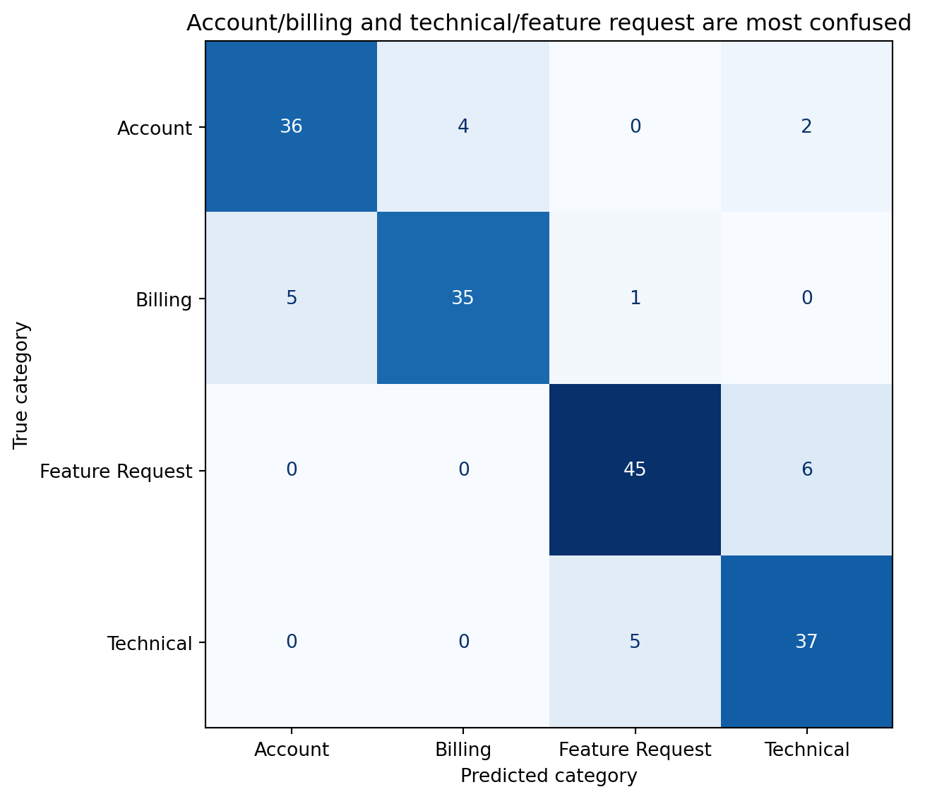
## Handling misclassifications: the confusion matrix {#sec-nlp-confusion}
Text classification errors aren't random; they cluster around categories with overlapping vocabulary. The confusion matrix reveals which categories the model confuses and why.
```{python}
#| label: fig-nlp-confusion
#| echo: true
#| fig-cap: "Confusion matrix for the ticket classifier. Off-diagonal cells reveal where vocabulary overlap causes misclassification — account and billing tickets share financial terms, while technical and feature request tickets share product terminology."
#| fig-alt: "A four-by-four confusion matrix with predicted category on the horizontal axis and true category on the vertical axis. Each cell is annotated with a count. Diagonal cells contain the largest numbers, showing correct predictions. The main off-diagonal confusions occur between account and billing tickets, and between technical and feature request tickets — categories that share overlapping vocabulary."
from sklearn.metrics import confusion_matrix, ConfusionMatrixDisplay

cm = confusion_matrix(y_test, y_pred_lr, labels=classes)

fig, ax = plt.subplots(figsize=(7, 6))
fig.patch.set_alpha(0)
ax.patch.set_alpha(0)
disp = ConfusionMatrixDisplay(cm, display_labels=[c.replace('_', ' ').title()
                                                    for c in classes])
disp.plot(ax=ax, cmap='Blues', colorbar=False)
ax.set_xlabel('Predicted category')
ax.set_ylabel('True category')
ax.set_title('Account/billing and technical/feature request are most confused')
plt.tight_layout()
plt.show()
```
The confusion pattern tells a story. Tickets about changing payment methods could plausibly be "billing" or "account." Tickets requesting an API endpoint could be "feature request" or "technical." A ticket mentioning "dashboard" could be a technical bug report or a feature request. These ambiguities aren't model failures — they're genuine ambiguities in the data that a human classifier would also struggle with. When categories overlap semantically, the model's error rate on those boundaries is a floor, not a ceiling.
## Discovering structure: topic modelling {#sec-nlp-topics}
Classification requires labelled data: someone had to assign each ticket to a category. But what if you have thousands of unlabelled tickets and want to discover what topics they cover? **Topic modelling** is the unsupervised equivalent: it discovers latent thematic structure in a corpus without any labels.
**Non-negative matrix factorisation** (NMF) decomposes the TF-IDF matrix $\mathbf{V}$ (documents × words) into two non-negative matrices: $\mathbf{W}$ (documents × topics) and $\mathbf{H}$ (topics × words):
$$
\mathbf{V} \approx \mathbf{W} \mathbf{H}
$$
Each row of $\mathbf{H}$ is a topic, represented as a non-negative weighting over words. Each row of $\mathbf{W}$ is a document, represented as a mixture of topics. The non-negativity constraint (all values ≥ 0) ensures that topics are additive: a document is a *sum* of topic contributions, never a subtraction. This produces interpretable topics where the top words in each topic tend to be semantically coherent.
If you've worked with dimensionality reduction (@sec-too-many-features), NMF should feel familiar. PCA also decomposes a matrix into lower-rank factors, but it allows negative values, which makes the components harder to interpret as "topics." NMF trades the optimality guarantees of PCA for interpretability, a worthwhile trade when the goal is understanding rather than compression.
```{python}
#| label: nlp-topic-model
#| echo: true
from sklearn.decomposition import NMF

# Use the full corpus (not just training set) for topic discovery
tfidf_full = TfidfVectorizer(ngram_range=(1, 2), stop_words='english',
                              max_features=2000)
X_topics = tfidf_full.fit_transform(tickets['text'])
topic_feature_names = tfidf_full.get_feature_names_out()

# Fit NMF with 4 topics (we happen to know there are 4 categories —
# in practice you'd try several values and evaluate coherence)
nmf = NMF(n_components=4, random_state=42, max_iter=500)
W = nmf.fit_transform(X_topics)
H = nmf.components_

print('Discovered topics (top 8 words each):\n')
for i, topic in enumerate(H):
    top_words = topic_feature_names[np.argsort(topic)[-8:][::-1]]
    print(f"  Topic {i}: {', '.join(top_words)}")
```
```{python}
#| label: fig-nlp-topic-category
#| echo: true
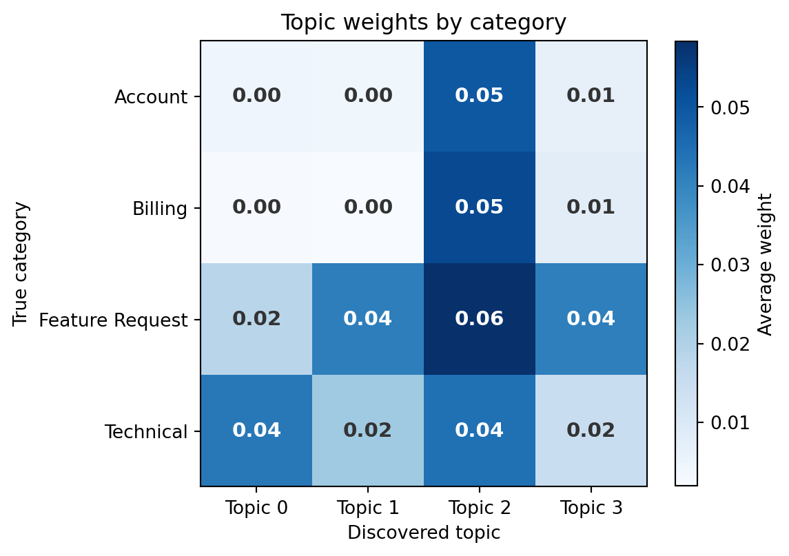
#| fig-cap: "Average topic weight by true category. Each cell shows the mean NMF topic weight for tickets in that category. Topics load unevenly across categories, revealing partial alignment between discovered topics and labelled ground truth."
#| fig-alt: "Heatmap with four rows (account, billing, feature request, technical) and four columns (Topic 0 through 3). Numeric weights are annotated in each cell. Each topic loads unevenly across categories — some topics concentrate on one category while others spread across two or more, showing partial but imperfect alignment between unsupervised topics and supervised labels."
# Map topics to categories
topic_weights = pd.DataFrame(W, columns=[f"Topic {i}" for i in range(4)])
topic_weights['category'] = tickets['category'].values

avg_weights = topic_weights.groupby('category').mean()

fig, ax = plt.subplots(figsize=(6, 5))
fig.patch.set_alpha(0)
ax.patch.set_alpha(0)
im = ax.imshow(avg_weights.values, cmap='Blues', aspect='equal')

ax.set_xticks(range(4))
ax.set_xticklabels(avg_weights.columns)
ax.set_yticks(range(len(avg_weights)))
ax.set_yticklabels([c.replace('_', ' ').title() for c in avg_weights.index])

# Add text annotations — use threshold for contrast
threshold = avg_weights.values.max() * 0.55
for i in range(len(avg_weights)):
    for j in range(4):
        val = avg_weights.values[i, j]
        ax.text(j, i, f'{val:.2f}', ha='center', va='center',
                fontsize=11, fontweight='bold',
                color='white' if val > threshold else '#333333')

ax.set_title('Topic weights by category')
ax.set_xlabel('Discovered topic')
ax.set_ylabel('True category')
plt.colorbar(im, ax=ax, label='Average weight', shrink=0.8)
plt.tight_layout()
plt.show()
```
@fig-nlp-topic-category shows that the unsupervised topics partially align with the known categories: some topics load unevenly across categories, concentrating weight on one or two. Others spread more broadly. This is typical: NMF discovers whatever structure exists in word co-occurrence patterns, and that structure doesn't always map one-to-one onto business categories. Cross-category vocabulary (words like "account," "team," and "update" that appear in multiple categories) blurs the boundaries. In practice, topic modelling is most useful when you *don't* have labels: exploring a large corpus of customer feedback to discover what themes emerge, before deciding how to categorise them.
::: {.callout-note}
## Engineering Bridge
Topic modelling serves a similar role to **log clustering** in operations. When you have millions of log lines and need to understand what's happening, you don't read them individually; you cluster them into patterns and examine the representative entries from each cluster. Tools like Elasticsearch's significant terms aggregation and log analysis platforms do this automatically. NMF topic modelling is the same idea applied to natural language: reduce a large, unstructured corpus to a manageable set of themes, each characterised by its most representative words. The output is a starting point for human investigation, just as log clusters are a starting point for root cause analysis.
:::
## Out-of-vocabulary words {#sec-nlp-vocabulary}
A text model's vocabulary is fixed at training time. Any word that appears in a new document but wasn't in the training corpus is simply ignored: it gets no column in the TF-IDF matrix and contributes nothing to the prediction. This is the **out-of-vocabulary** (OOV) problem, and it's the text equivalent of encountering a feature value at inference time that the model never saw during training.
```{python}
#| label: nlp-oov-demo
#| echo: true
#| code-fold: true
#| code-summary: "Expand to see OOV prediction code"
# The vectoriser was fit on training data — it knows those words
training_vocab_size = len(vectoriser.vocabulary_)

# These tickets use words the model may not have seen
new_tickets = [
    'The Kubernetes deployment keeps failing with OOMKilled errors',
    'Can we get a GraphQL endpoint instead of REST',
    'Our SAML configuration is rejecting assertions from Okta',
]

X_new = vectoriser.transform(new_tickets)

# How many tokens does the vectoriser actually recognise?
analyser = vectoriser.build_analyzer()
for i, ticket in enumerate(new_tickets):
    n_recognised = X_new[i].nnz
    tokens = analyser(ticket)
    print(f"Ticket: '{ticket[:60]}...'")
    print(f"  Tokens: {len(tokens)}, recognised by model: {n_recognised}\n")

# What does the model predict?
predictions = lr.predict(X_new)
probabilities = lr.predict_proba(X_new)

for ticket, pred, probs in zip(new_tickets, predictions, probabilities):
    confidence = probs.max()
    print(f"  Prediction: {pred:16s} (confidence: {confidence:.1%})")
    print(f"  '{ticket[:60]}...'\n")
```
The model predicts *something* for every input; it never says "I don't know." But when most of the input's vocabulary is out-of-vocabulary, the prediction is based on the few surviving words, which may not capture the ticket's actual meaning. A Kubernetes deployment failure is a technical issue, but if the model hasn't seen "Kubernetes" or "OOMKilled" in training, it's guessing from whatever residual words survived the vectoriser.
This highlights a structural limitation of bag-of-words approaches. The model's world is bounded by its training vocabulary. New products, technologies, and jargon require retraining, or a representation strategy that generalises beyond the specific words seen in training, which is where word embeddings and language models (beyond the scope of this book) provide significant advantages.
::: {.callout-tip}
## Author's Note
The OOV problem reframed how I think about the relationship between a model and its training data. In software, a well-designed function handles any valid input: you don't expect `sort()` to fail on a list it hasn't seen before. But a text classifier is fundamentally different: it can only reason about words it was trained on, and the set of possible words is open-ended. The model isn't a general-purpose function — it's a lookup table with interpolation, and it breaks silently at the edges of its vocabulary. This is why monitoring text models in production requires tracking not just prediction confidence but *vocabulary coverage*, the fraction of input words that the model actually recognises. A drop in coverage is an early signal that the model's world has become too small.
:::
## Production considerations {#sec-nlp-production}
Deploying a text classifier involves several engineering challenges that don't appear in the notebook.
### The vectoriser is part of the model {#sec-nlp-vectoriser-deployment}
The TF-IDF vectoriser, with its learned vocabulary, IDF weights, and preprocessing rules, is as much a part of the deployed system as the logistic regression weights. If you serialise the classifier but not the vectoriser, or if you rebuild the vectoriser on different data, the feature indices won't align and the model will produce garbage. The `Pipeline` abstraction in scikit-learn (@sec-model-serialisation) handles this by bundling the vectoriser and classifier into a single serialisable object.
### Preprocessing must be identical {#sec-nlp-preprocessing-parity}
Any text preprocessing applied during training (lowercasing, stop word removal, tokenisation rules) must be applied identically at inference time. A common production bug is training with scikit-learn's English stop word list but deploying behind a different preprocessing pipeline (perhaps a custom microservice) that uses a slightly different stop word list. The model sees different features at inference time and accuracy degrades silently.
### Latency and vocabulary size {#sec-nlp-latency}
A TF-IDF vectoriser with bigrams on a large corpus can produce hundreds of thousands of features. The sparse matrix–vector multiplication for logistic regression is fast, $O(\text{nnz})$ where `nnz` is the number of non-zero entries in the document's vector, meaning cost scales with how many words the document actually uses, not the total vocabulary size. But the vectoriser's tokenisation and hashing step can be the latency bottleneck. For high-throughput applications, consider `HashingVectorizer`, which maps words to features using a hash function rather than a vocabulary lookup, sacrificing interpretability for constant memory and no fitting step.
### Retraining cadence {#sec-nlp-retraining}
As the product evolves and customers adopt new terminology, the model's vocabulary drifts out of date. A ticket about a feature that was launched after training ("the new Workflows feature isn't triggering") contains a key word the model doesn't recognise. Unlike the gradual distribution drift in churn prediction (@sec-churn-pipeline) or the adversarial drift in fraud detection (@sec-fraud-drift), vocabulary drift in NLP is driven by product changes and industry evolution. Monitoring vocabulary coverage (the fraction of input tokens that appear in the model's vocabulary) provides an early warning signal for when retraining is needed.
### Monitoring vocabulary coverage {#sec-nlp-coverage-monitoring}
Vocabulary coverage is straightforward to compute: tokenise the incoming text using the same analyser the model uses, then ask what fraction of those tokens appear in the vectoriser's learned vocabulary. Because the analyser is configured with bigrams, "token" here means both unigrams and bigrams, not literal words, so coverage is measured over tokens rather than over individual words. The arithmetic is two lines; the operational discipline is choosing a threshold and wiring the metric into your alerting.
```{python}
#| label: nlp-coverage-function
#| echo: true
def vocabulary_coverage(texts, vectoriser):
    """Fraction of tokens in `texts` that appear in the vectoriser's vocabulary."""
    analyser = vectoriser.build_analyzer()
    vocab = vectoriser.vocabulary_  # token -> index mapping
    total, in_vocab = 0, 0
    for text in texts:
        tokens = analyser(text)
        total += len(tokens)
        in_vocab += sum(1 for t in tokens if t in vocab)
    return in_vocab / total if total else 0.0

# Baseline: coverage on the held-out test set (in-distribution by construction)
baseline = vocabulary_coverage(X_test_text, vectoriser)
print(f"Baseline coverage on held-out test set: {baseline:.1%}")
```
A reasonable alert threshold is **5 percentage points below the baseline**, sustained over enough traffic to rule out short-term sampling noise. Below that, something has shifted: a product launch has introduced new feature names, a marketing campaign is bringing in users from a new domain, or the support team has changed how they describe issues. Each cause has a different remediation, but you only know which one applies if you are watching the metric.
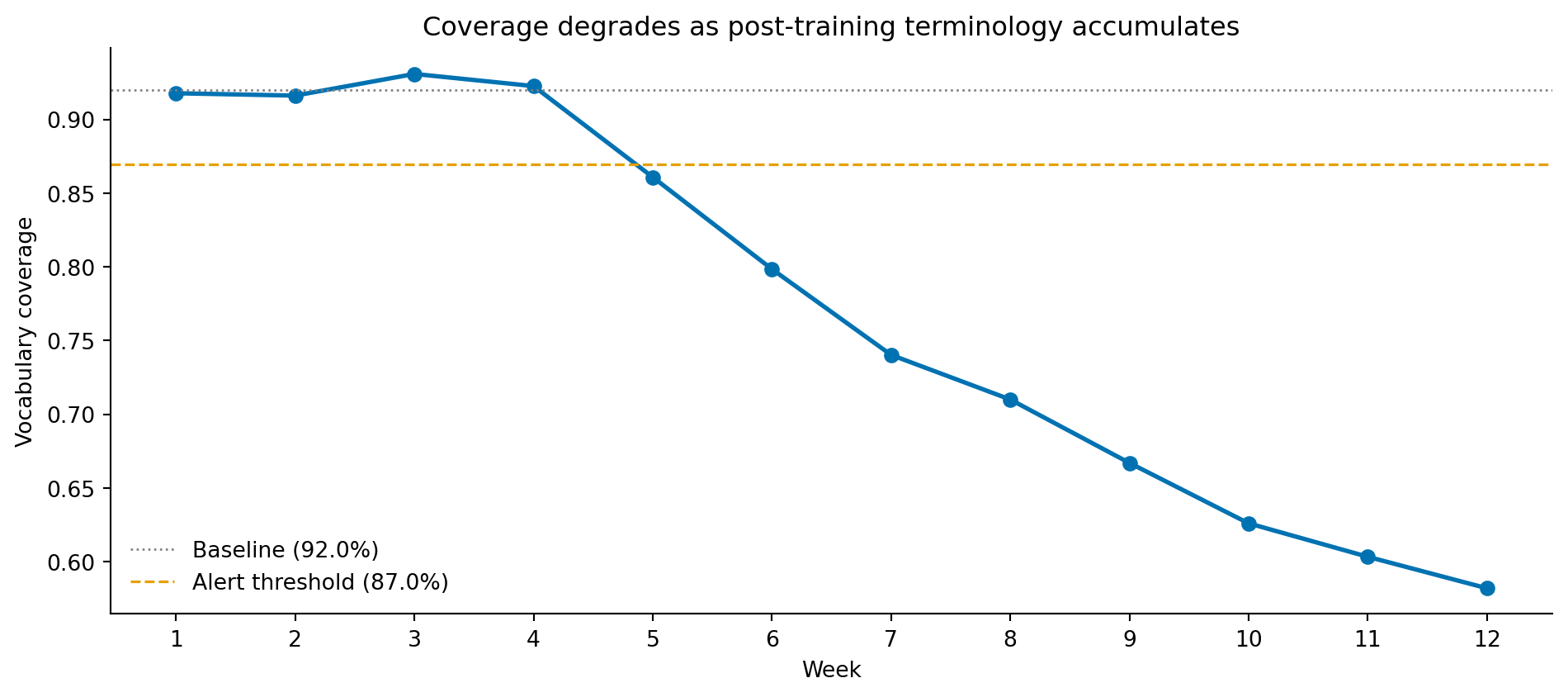
To make the alert concrete, simulate twelve weeks of incoming tickets where weeks 5–12 progressively introduce new product vocabulary (`workflows`, `autopilot`, `copilot`, `snapshots`) that did not exist in training.
```{python}
#| label: fig-coverage-drift
#| echo: true
#| fig-cap: "Weekly vocabulary coverage as new product terms are introduced. Coverage holds steady for the first four weeks, then drops as the proportion of tickets containing post-training terminology climbs. The dashed line marks a 5-percentage-point drop from baseline — a reasonable retraining trigger."
#| fig-alt: "Line chart of vocabulary coverage by week from week 1 to week 12. Coverage hovers around 92% for the first four weeks, then declines steeply week-on-week, reaching roughly 58% by week 12. A horizontal dashed orange line at baseline minus 5 percentage points is crossed at week 5, marking when an automated alert would fire."
new_terms = ['workflows', 'autopilot', 'copilot', 'snapshots']
weekly = []
for week in range(1, 13):
    drift_fraction = max(0, (week - 4) * 0.10)  # weeks 1-4 clean, then climbing
    n = 200
    drift_n = int(n * drift_fraction)
    sampled = X_test_text.sample(n, random_state=week, replace=True).tolist()
    for i in range(drift_n):
        sampled[i] = sampled[i] + ' ' + ' '.join(rng.choice(new_terms, size=3))
    weekly.append(vocabulary_coverage(sampled, vectoriser))

fig, ax = plt.subplots(figsize=(10, 4.5))
fig.patch.set_alpha(0)
ax.patch.set_alpha(0)
weeks = list(range(1, 13))
ax.plot(weeks, weekly, 'o-', color='#0072B2', linewidth=2)
ax.axhline(baseline, color='grey', linestyle=':', linewidth=1, label=f'Baseline ({baseline:.1%})')
ax.axhline(baseline - 0.05, color='#E69F00', linestyle='--', linewidth=1.2,
           label=f'Alert threshold ({baseline - 0.05:.1%})')
ax.set_xlabel('Week')
ax.set_ylabel('Vocabulary coverage')
ax.set_title('Coverage degrades as post-training terminology accumulates')
ax.set_xticks(weeks)
ax.legend(frameon=False, loc='lower left')
ax.spines[['top', 'right']].set_visible(False)
plt.tight_layout()
plt.show()
```
When the alert fires, the response is not automatic; the right action depends on diagnosing *which* tokens are missing. Three patterns recur. If the new tokens are **product names** (a feature that did not exist in training), the fix is a retraining run on data that includes the post-launch tickets. If the new tokens are **domain jargon** that the team uses but the customer does not — the inverse problem — adding those terms to a domain-specific stop-word list or a custom token mapping can suffice without a full retrain. If the missing tokens are **misspellings or formatting noise** (`emaill`, `loggin`), the upstream fix is a richer preprocessing pipeline (stemming, character-level fallback) rather than retraining. Inspecting the top-N out-of-vocabulary tokens in the offending batch is what tells you which case you are in. This kind of diagnostic loop is exactly what makes vocabulary coverage a useful production metric rather than a vanity number on a dashboard.
## Summary {#sec-nlp-summary}
1. **Text representation is the core challenge.** Bag of words and TF-IDF convert variable-length text into fixed-length numerical vectors by treating documents as collections of words and weighting by distinctiveness. Word order is lost, but for many classification tasks the informative signal lies in *which* words appear, not their arrangement.
2. **Linear models work well for text.** Logistic regression on TF-IDF features is a strong baseline for text classification because the high dimensionality and sparsity of text data suit linear decision boundaries with L2 regularisation. Tree-based models, which split on individual features, struggle with the extreme sparsity.
3. **Topic modelling discovers structure without labels.** NMF decomposes the document-term matrix into interpretable topics — distributions over words — that reveal thematic structure in a corpus. This is unsupervised dimensionality reduction applied to text.
4. **The vocabulary is a hard boundary.** Words not seen during training are invisible to the model. Monitoring vocabulary coverage in production is essential for detecting when the model's representation has become stale.
5. **The vectoriser is part of the model.** Text preprocessing and vectorisation must be identical at training and inference time. Serialise the full pipeline, not just the classifier weights.
## Exercises {#sec-nlp-exercises}
1. Replace logistic regression with a Complement Naive Bayes classifier (`ComplementNB` from scikit-learn), which is designed to work with TF-IDF features. Compare accuracy and per-class F1 scores. Naive Bayes assumes features are conditionally independent given the class — why might this assumption be *more* reasonable for bag-of-words text features than for typical structured data features? (Note: `MultinomialNB` expects non-negative count data and is an antipattern with TF-IDF vectors; `ComplementNB` handles the TF-IDF weighting correctly.)
2. Experiment with the `max_features` parameter of `TfidfVectorizer`, which limits the vocabulary to the N most frequent terms. Try values of 500, 1,000, 2,000, and 5,000. Plot accuracy against vocabulary size. At what point does adding more features stop helping? What does this tell you about the effective dimensionality of the classification problem?
3. The topic model used 4 components because we knew there were 4 categories. Refit NMF with 3, 5, 6, and 8 components. Examine the top words for each topic. What happens when you use too few topics (themes get merged)? Too many (themes get split or noise topics emerge)? How would you choose the number of topics when you don't have ground-truth labels?
4. **Conceptual:** A colleague suggests improving the ticket classifier by adding metadata features alongside the text — time of day, customer tenure, product tier, and browser type. How would you combine these structured features with TF-IDF text features in a single model? What preprocessing challenges arise from mixing dense low-dimensional metadata with sparse high-dimensional text features?
5. **Conceptual:** The bag-of-words model treats "the API is not working" and "the API is working" as nearly identical documents (they share most words and differ only by "not"). In what business contexts would this be a serious problem? How might you mitigate it without moving to deep learning — for instance, by engineering specific features or adjusting the tokenisation strategy?