20  Testing data science code

20.1 The assert that doesn’t work

You know how to write tests. You’ve written thousands of them: unit tests that check return values, integration tests that verify API contracts, end-to-end tests that simulate user workflows. Your CI pipeline runs them on every push. A red build means something is broken. A green build means your code does what you said it would.

Now try writing a test for a machine learning model:

import numpy as np
import pandas as pd
from sklearn.ensemble import RandomForestClassifier
from sklearn.model_selection import train_test_split

rng = np.random.default_rng(42)
X = rng.normal(0, 1, (500, 5))
y = (X[:, 0] + 0.5 * X[:, 1] + rng.normal(0, 0.3, 500) > 0).astype(int)

X_train, X_test, y_train, y_test = train_test_split(
    X, y, test_size=0.2, random_state=42
)

model = RandomForestClassifier(n_estimators=100, random_state=42)
model.fit(X_train, y_train)

accuracy = model.score(X_test, y_test)
print(f"Accuracy: {accuracy:.4f}")

# This is a test... but what should the expected value be?
assert accuracy > 0.80, f"Model accuracy {accuracy:.4f} below threshold"

Accuracy: 0.9200

The assertion passes, but something about it feels wrong. In software testing, expected values come from specifications: the function should return 35.96 because the invoice maths says so. Here, the threshold of 0.80 came from… where? You picked it because it seemed reasonable. If the accuracy comes back at 0.79, is the model broken? Is the data different? Is the random seed behaving differently on this machine? You’re no longer testing correctness; you’re testing “good enough”, and the boundary between those two is fuzzy.

This is the fundamental tension in testing data science code. Your engineering instincts are exactly right: untested code is untrustworthy code, but the testing patterns you know were designed for deterministic systems. Data science code produces approximate, probabilistic, data-dependent outputs. You need a different testing vocabulary, built on the same disciplined foundations.

NoteEngineering Bridge

In web development, you test against a specification: the API contract says GET /users/42 returns a JSON object with an id field. In data science, there is often no specification: the model’s behaviour is the specification, discovered empirically from data. This is closer to testing a search engine’s relevance ranking than testing a CRUD endpoint. You can’t assert exact outputs, but you can assert properties: results should be ordered by relevance, the top result should be relevant, and adding a typo shouldn’t completely destroy the rankings. The shift is from exact-output testing to behavioural testing: asserting what kind of answer you expect rather than which exact answer. (This is distinct from property-based testing in the Hypothesis/QuickCheck sense, where a framework generates random inputs to find counterexamples, a complementary technique worth exploring separately.)

20.2 Testing the deterministic parts first

Before wrestling with probabilistic outputs, recognise that most data science code is deterministic. Data cleaning functions, feature engineering transforms, and preprocessing pipelines take a DataFrame in and produce a DataFrame out. These are ordinary functions that deserve ordinary tests.

def compute_recency_features(
    df: pd.DataFrame,
    reference_date: pd.Timestamp,
) -> pd.DataFrame:
    """Compute days-since features relative to a reference date."""
    result = df.copy()
    result['days_since_last_order'] = (
        (reference_date - df['last_order_date']).dt.days
    )
    result['days_since_signup'] = (
        (reference_date - df['signup_date']).dt.days
    )
    result['order_recency_ratio'] = (
        result['days_since_last_order'] / result['days_since_signup']
    )
    return result


# --- Tests ---
def test_recency_features():
    ref_date = pd.Timestamp('2025-01-15')
    test_data = pd.DataFrame({
        'last_order_date': [pd.Timestamp('2025-01-10'),
                            pd.Timestamp('2024-12-15')],
        'signup_date': [pd.Timestamp('2024-01-15'),
                        pd.Timestamp('2023-01-15')],
    })

    result = compute_recency_features(test_data, ref_date)

    # Exact assertions — these are deterministic computations
    assert result['days_since_last_order'].tolist() == [5, 31]
    assert result['days_since_signup'].tolist() == [366, 731]
    np.testing.assert_allclose(
        result['order_recency_ratio'].values,
        [5 / 366, 31 / 731],
    )

    # Structural assertions — output shape and columns
    assert list(result.columns) == [
        'last_order_date', 'signup_date',
        'days_since_last_order', 'days_since_signup',
        'order_recency_ratio',
    ]

test_recency_features()
print('All deterministic tests passed.')

All deterministic tests passed.

These tests use exact equality because the computations are exact. Date arithmetic, string manipulation, joins, filters, aggregations: all deterministic, all testable in the same way you’d test any utility function. The advice here is simple: extract your data transformations into pure functions and test them like any other code. The fact that they happen to operate on DataFrames rather than strings or integers doesn’t change the testing discipline.

Treat pytest as your primary testing framework. The standard project layout works for data science exactly as it works for application code: a tests/ directory, one test module per source module, fixtures for shared test data. In a real project, these tests would live in separate files:

# tests/test_features.py (not executed — illustrative)
import pytest
import pandas as pd

@pytest.fixture
def sample_orders():
    return pd.DataFrame({
        "last_order_date": pd.to_datetime(
            ["2025-01-10", "2024-12-15"]
        ),
        "signup_date": pd.to_datetime(
            ["2024-01-15", "2023-01-15"]
        ),
    })

def test_recency_days_are_positive(sample_orders):
    result = compute_recency_features(
        sample_orders, pd.Timestamp("2025-01-15")
    )
    assert (result["days_since_last_order"] >= 0).all()
    assert (result["days_since_signup"] >= 0).all()

def test_recency_ratio_bounded(sample_orders):
    result = compute_recency_features(
        sample_orders, pd.Timestamp("2025-01-15")
    )
    # Ratio should be between 0 and 1 for customers
    # who ordered after signup
    assert (result["order_recency_ratio"] >= 0).all()
    assert (result["order_recency_ratio"] <= 1).all()

Notice that the second test checks a property (the ratio is between 0 and 1) rather than an exact value. This is a preview of the pattern we’ll use increasingly for statistical code.

20.3 Approximate equality and tolerances

When code involves floating-point arithmetic (and nearly all data science code does), exact equality breaks down. Two mathematically equivalent computations can produce slightly different floating-point results due to the non-associativity of IEEE 754 arithmetic: different execution orders, compiler optimisations, or BLAS implementations can produce results that diverge in the last few significant digits. (Section 16.5 covers the related but distinct problem of non-determinism from pseudorandom number generators; here the source of variation is floating-point arithmetic itself, not randomness.)

NumPy provides np.testing.assert_allclose for this purpose. It checks that values are equal within a relative tolerance (rtol) and an absolute tolerance (atol):

# These are mathematically equal but differ at machine precision
a = 0.1 + 0.2
b = 0.3
print(f"0.1 + 0.2 = {a!r}")
print(f"0.3       = {b!r}")
print(f"Equal?      {a == b}")

# assert_allclose handles this gracefully
np.testing.assert_allclose(a, b, rtol=1e-10)
print('assert_allclose passed (rtol=1e-10)')

0.1 + 0.2 = 0.30000000000000004
0.3       = 0.3
Equal?      False
assert_allclose passed (rtol=1e-10)

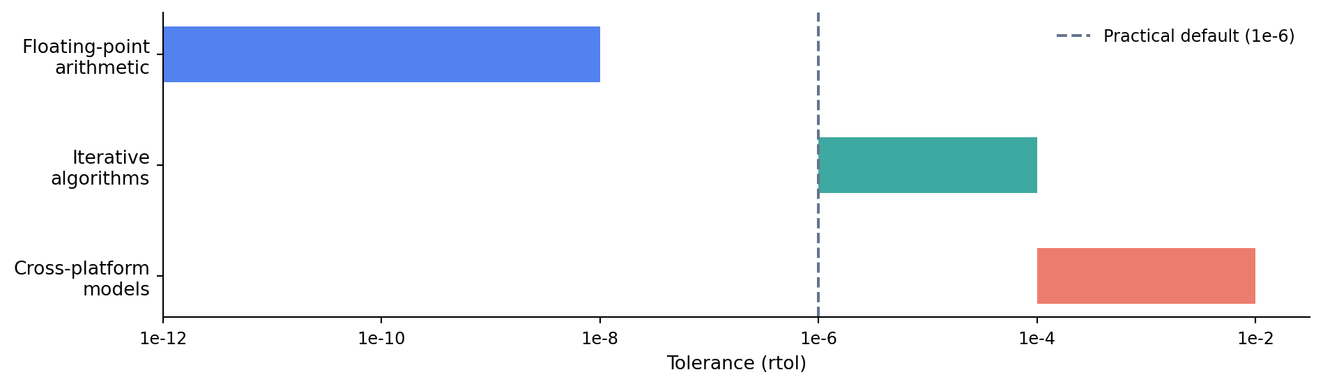
The choice of tolerance matters. Too tight and your tests become flaky, failing on different machines or library versions because of insignificant numerical differences. Too loose and your tests miss genuine bugs. Figure 20.1 shows the practical ranges for different kinds of computation.

import matplotlib.pyplot as plt
import numpy as np

fig, ax = plt.subplots(figsize=(10, 3))

categories = [
    'Floating-point\narithmetic',
    'Iterative\nalgorithms',
    'Cross-platform\nmodels',
]
starts = [1e-12, 1e-6, 1e-4]
ends = [1e-8, 1e-4, 1e-2]
colours = ['#0072B2', '#009E73', '#D55E00']  # Okabe-Ito: colour-blind safe

for i, (cat, s, e, c) in enumerate(
    zip(categories, starts, ends, colours)
):
    ax.barh(
        i, np.log10(e) - np.log10(s),
        left=np.log10(s), height=0.5, color=c, alpha=0.8,
    )

ax.set_yticks(range(len(categories)))
ax.set_yticklabels(categories, fontsize=10)
ax.set_xlabel('Tolerance (rtol) — logarithmic scale', fontsize=10)
ax.set_xticks(range(-12, 0, 2))
ax.set_xticklabels(
    [f'1e{x}' for x in range(-12, 0, 2)], fontsize=9
)
ax.axvline(
    x=-6, color='#64748b', linestyle='--',
    linewidth=1.5, label='Practical default (1e-6)',
)
ax.text(
    -5.8, 2.55, '1e-6\ndefault', fontsize=8,
    color='#64748b', va='top',
)
ax.legend(fontsize=9, frameon=False)
ax.spines[['top', 'right']].set_visible(False)
ax.invert_yaxis()
fig.patch.set_alpha(0)
ax.patch.set_alpha(0)
plt.tight_layout()
plt.show()

Figure 20.1: Tolerance guidelines for different types of numerical computation. Tighter tolerances catch more bugs but risk flaky tests; looser tolerances are more robust across platforms.

For computations where the expected value may be close to zero, rtol alone is insufficient: the relative comparison divides by a near-zero denominator, making even tiny absolute differences look large. In those cases, set both rtol and atol (e.g., rtol=1e-10, atol=1e-12).

from sklearn.linear_model import LogisticRegression
from sklearn.datasets import make_classification

X_tol, y_tol = make_classification(
    n_samples=200, n_features=5, random_state=42
)

# Train the same model twice — numerically identical to near-machine
# precision on the same platform, because the same deterministic solver
# runs on the same data (not because of the convergence tolerance)
model_a = LogisticRegression(
    random_state=42, max_iter=200
).fit(X_tol, y_tol)
model_b = LogisticRegression(
    random_state=42, max_iter=200
).fit(X_tol, y_tol)

np.testing.assert_allclose(
    model_a.predict_proba(X_tol),
    model_b.predict_proba(X_tol),
    rtol=1e-10,
)
print('Same-machine reproducibility: passed (rtol=1e-10)')

# Note: same-machine equality is almost guaranteed for a deterministic solver.
# The real test is cross-platform: running on a different OS, BLAS build, or
# CPU architecture. For that, use a looser tolerance (rtol=1e-5 or 1e-6) and
# compare against stored fixture values rather than recomputing on the same run.

Same-machine reproducibility: passed (rtol=1e-10)

TipAuthor’s Note

Flaky tests in data science code are often not flaky at all — they’re exposing legitimate numerical non-determinism that you didn’t account for. Different CPU architectures use different BLAS implementations, which produce different optimisation paths, which yield slightly different coefficients. A test that compares to six decimal places will fail intermittently across machines, and the instinct is to look for a code bug. But the “bug” is that floating-point optimisation is not bitwise reproducible across hardware. The fix is to choose an appropriate tolerance, rtol=1e-6 for anything involving optimisation, and only tighten it when you have a reason to. Numerical tolerance is a design decision, not a sign of sloppiness.

20.4 Behavioural tests for models

You can’t assert that a model returns a specific prediction: the exact output depends on the training data, the random seed, and the library version. But you can assert how the model should behave. These behavioural tests check properties of the model’s outputs rather than their exact values.

There are four patterns that cover most cases. Each is worth understanding individually before we combine them in the worked example.

20.4.1 Smoke tests

Smoke tests check that the model runs without crashing and produces outputs of the expected shape and type. These catch packaging errors, missing dependencies, and serialisation bugs:

from sklearn.ensemble import GradientBoostingClassifier
from sklearn.datasets import make_classification

X_smoke, y_smoke = make_classification(
    n_samples=300, n_features=5, random_state=42
)

smoke_model = GradientBoostingClassifier(
    n_estimators=50, random_state=42
)
smoke_model.fit(X_smoke, y_smoke)

# Smoke tests
X_new = np.random.default_rng(99).normal(0, 1, (10, 5))
predictions = smoke_model.predict(X_new)
probabilities = smoke_model.predict_proba(X_new)

assert predictions.shape == (10,), 'Wrong prediction shape'
assert probabilities.shape == (10, 2), 'Wrong probability shape'
assert set(predictions).issubset({0, 1}), 'Unexpected labels'
assert np.all(probabilities >= 0), 'Negative probabilities'
assert np.allclose(probabilities.sum(axis=1), 1.0), (
    "Probabilities don't sum to 1"
)
print('All smoke tests passed.')

All smoke tests passed.

20.4.2 Directional tests

Directional tests (also called perturbation tests) check that changing an input in a known direction produces the expected change in output. If you increase a customer’s spending, a churn model should predict lower churn probability. If you increase an error rate, an incident model should predict higher incident probability:

from sklearn.ensemble import GradientBoostingClassifier
from scipy.special import expit  # logistic sigmoid: maps log-odds to [0, 1]

# Train an incident prediction model
rng = np.random.default_rng(42)
n = 800
incident_features = pd.DataFrame({
    'error_pct': np.clip(rng.normal(2, 1.5, n), 0, None),
    'request_rate': rng.exponential(100, n),
    'p99_latency_ms': rng.lognormal(4, 0.8, n),  # lognormal: latencies are right-skewed
})
log_odds = (
    -3.5
    + 0.4 * incident_features['error_pct']
    + 0.005 * incident_features['request_rate']
)
incident_target = rng.binomial(1, expit(log_odds))

incident_model = GradientBoostingClassifier(
    n_estimators=100, random_state=42
).fit(incident_features, incident_target)

# Directional test: increasing error_pct should increase
# incident probability
baseline = pd.DataFrame({
    'error_pct': [2.0],
    'request_rate': [100.0],
    'p99_latency_ms': [50.0],
})
perturbed = baseline.copy()
perturbed['error_pct'] = 8.0  # much higher error rate

p_baseline = incident_model.predict_proba(baseline)[0, 1]
p_perturbed = incident_model.predict_proba(perturbed)[0, 1]

assert p_perturbed > p_baseline, (
    f"Higher error rate should increase incident probability, "
    f"but {p_perturbed:.3f} <= {p_baseline:.3f}"
)
print(f"Baseline (error=2%):  {p_baseline:.3f}")
print(f"Perturbed (error=8%): {p_perturbed:.3f}")
print('Directional test passed.')

Baseline (error=2%):  0.043
Perturbed (error=8%): 0.891
Directional test passed.

20.4.3 Invariance tests

Invariance tests check that features which should not affect the output genuinely do not. A credit scoring model shouldn’t change its prediction when you vary the applicant’s name. A fraud detection model shouldn’t depend on the transaction ID. This pattern catches both data leakage bugs (the model accidentally learned from an identifier) and fairness issues (the model responds to a protected attribute):

# Add a column that the model should NOT depend on
baseline_with_id = baseline.copy()
baseline_with_id['server_id'] = 'web-eu-042'

altered_id = baseline_with_id.copy()
altered_id['server_id'] = 'web-us-999'

# The model was trained on numeric features only, so server_id
# should be irrelevant. Verify by predicting on the shared columns.
feature_cols = ['error_pct', 'request_rate', 'p99_latency_ms']
p_original = incident_model.predict_proba(
    baseline_with_id[feature_cols]
)[0, 1]
p_altered = incident_model.predict_proba(
    altered_id[feature_cols]
)[0, 1]

assert p_original == p_altered, (
    'Changing server_id altered the prediction — '
    'possible data leakage through an identifier'
)
print(f"Prediction with server_id='web-eu-042': {p_original:.3f}")
print(f"Prediction with server_id='web-us-999': {p_altered:.3f}")
print('Invariance test passed.')

Prediction with server_id='web-eu-042': 0.043
Prediction with server_id='web-us-999': 0.043
Invariance test passed.

In a real system, the invariance test becomes more meaningful when the irrelevant column is present in the training data, for example checking that a model trained on features including user_id doesn’t actually depend on it. Here the test is straightforward because we excluded server_id from training. The pattern matters most when you’re not sure what the model learned.

20.4.4 Minimum performance tests

Minimum performance tests set a floor that the model must exceed. The threshold should come from a meaningful baseline: the performance of a simple heuristic, a previous model version, or a dummy classifier, not from an arbitrary number:

from sklearn.dummy import DummyClassifier
from sklearn.model_selection import cross_val_score

# Establish a meaningful baseline. "stratified" preserves
# the class distribution, giving a non-trivial baseline even
# with imbalanced classes (unlike "most_frequent", which
# predicts everything as the majority class and produces
# F1 = 0 for the minority class)
dummy = DummyClassifier(strategy='stratified', random_state=42)
dummy_scores = cross_val_score(
    dummy, incident_features, incident_target,
    cv=5, scoring='roc_auc',
)

# cross_val_score clones the estimator and refits from scratch
# on each fold — the existing fitted state is ignored
model_scores = cross_val_score(
    incident_model, incident_features, incident_target,
    cv=5, scoring='roc_auc',
)

print(f"Dummy baseline AUC: "
      f"{dummy_scores.mean():.3f} ± {dummy_scores.std():.3f}")
print(f"Model AUC:          "
      f"{model_scores.mean():.3f} ± {model_scores.std():.3f}")

# The model must meaningfully outperform the dummy
assert model_scores.mean() > dummy_scores.mean() + 0.05, (
    'Model does not meaningfully outperform '
    'the stratified dummy baseline'
)
print('Minimum performance test passed.')

Dummy baseline AUC: 0.518 ± 0.026
Model AUC:          0.623 ± 0.053
Minimum performance test passed.

NoteEngineering Bridge

These four patterns map to testing concepts you already use, though some analogies are closer than others. Smoke tests are health checks, the equivalent of hitting /healthz after a deployment. Directional tests are like testing that a rate limiter actually limits: when you double the request rate, the rejection count should increase. You don’t check the exact count, but you verify the direction. Invariance tests are like checking that an authorisation decision doesn’t depend on the X-Request-ID header; the request ID should be irrelevant to the outcome. Minimum performance tests are closest to SLO assertions: the service must maintain at least 99.9% availability, or the model must beat a meaningful baseline, say the stratified dummy’s AUC plus a margin that makes the model worth deploying.

20.5 Testing for data leakage

Data leakage (when information from the test set or the future leaks into training) is the most dangerous class of data science bug. It’s dangerous because the model appears to work better than it should: accuracy goes up, metrics look impressive, and nobody suspects a problem until the model fails in production. Here we focus on catching leakage in the data itself.

A temporal leakage test verifies that your train/test split respects time ordering. If you’re predicting next month’s churn, the training data must not include features computed from next month’s activity:

rng = np.random.default_rng(42)

# Simulate a dataset with temporal structure
n = 1000
events = pd.DataFrame({
    'event_date': pd.date_range(
        '2024-01-01', periods=n, freq='D'
    ),
    'revenue': rng.exponential(50, n),
    'user_count': rng.poisson(500, n),
})

# Define the prediction target date
prediction_date = pd.Timestamp('2024-10-01')

# Split: train on data before prediction_date, test on data after
train = events[events['event_date'] < prediction_date]
test = events[events['event_date'] >= prediction_date]

# Assert no temporal overlap
assert train['event_date'].max() < test['event_date'].min(), (
    'Temporal leakage: training data overlaps with test data'
)

# Assert test set starts at the expected boundary
assert test['event_date'].min() == prediction_date, (
    "Test set doesn't start at prediction_date"
)

# Assert all rows are accounted for
assert len(train) + len(test) == len(events), (
    'Rows lost during splitting'
)

print(f"Train: {train['event_date'].min().date()} to "
      f"{train['event_date'].max().date()} ({len(train)} rows)")
print(f"Test:  {test['event_date'].min().date()} to "
      f"{test['event_date'].max().date()} ({len(test)} rows)")
print('Temporal leakage test passed.')

Train: 2024-01-01 to 2024-09-30 (274 rows)
Test:  2024-10-01 to 2026-09-26 (726 rows)
Temporal leakage test passed.

A target leakage test checks that none of your features are derived from the target variable. This often happens subtly: a feature that is a near-perfect proxy for the label because it was computed from the same underlying data. The code block below intentionally triggers an assertion failure to demonstrate the detection pattern; the error output is expected:

from sklearn.ensemble import RandomForestClassifier
from sklearn.model_selection import cross_val_score

rng = np.random.default_rng(42)
n = 500

# Create a dataset where one feature leaks the target
leak_features = pd.DataFrame({
    'legitimate_feature_1': rng.normal(0, 1, n),
    'legitimate_feature_2': rng.normal(0, 1, n),
    'total_refund_amount': rng.exponential(10, n),
})
leak_target = (
    leak_features['total_refund_amount'] > 15
).astype(int)  # leaky!

# A suspiciously high cross-validation score is a red flag
rf = RandomForestClassifier(n_estimators=50, random_state=42)
scores = cross_val_score(
    rf, leak_features, leak_target, cv=5, scoring='accuracy'
)
print(f"CV accuracy with all features: {scores.mean():.3f}")

# Drop the suspect feature and compare
scores_clean = cross_val_score(
    rf,
    leak_features[['legitimate_feature_1',
                    'legitimate_feature_2']],
    leak_target, cv=5, scoring='accuracy',
)
print(f"CV accuracy without suspect:   {scores_clean.mean():.3f}")

accuracy_drop = scores.mean() - scores_clean.mean()
assert accuracy_drop < 0.15, (
    f"Dropping 'total_refund_amount' reduced accuracy by "
    f"{accuracy_drop:.1%} — possible target leakage. "
    f"Investigate before proceeding."
)
# This assertion WILL fail — demonstrating leakage detection
print(f"Accuracy drop: {accuracy_drop:.1%}")

CV accuracy with all features: 1.000
CV accuracy without suspect:   0.730

---------------------------------------------------------------------------
AssertionError                            Traceback (most recent call last)
Cell In[11], line 34
     31 print(f"CV accuracy without suspect:   {scores_clean.mean():.3f}")
     33 accuracy_drop = scores.mean() - scores_clean.mean()
---> 34 assert accuracy_drop < 0.15, (
     35     f"Dropping 'total_refund_amount' reduced accuracy by "
     36     f"{accuracy_drop:.1%} — possible target leakage. "
     37     f"Investigate before proceeding."
     38 )
     39 # This assertion WILL fail — demonstrating leakage detection
     40 print(f"Accuracy drop: {accuracy_drop:.1%}")

AssertionError: Dropping 'total_refund_amount' reduced accuracy by 27.0% — possible target leakage. Investigate before proceeding.

The pattern is straightforward: if removing a single feature causes a dramatic drop in performance, that feature is doing suspiciously heavy lifting. It may be legitimate — some features really are that predictive — but it warrants investigation. In this case the assertion fails because total_refund_amount is a direct proxy for the target, exactly the kind of leakage we want to catch.

20.6 Data validation tests

Models fail silently when their input data drifts from what they were trained on. A column that was never null during training starts arriving with nulls. A categorical feature gains a new level. Numeric values shift because an upstream system changed its units. The model keeps returning predictions — they’re just wrong.

Data validation tests catch these problems at the pipeline boundary, before the data reaches the model. Think of them as contract tests for your data:

def validate_model_input(df: pd.DataFrame) -> list[str]:
    """Validate a DataFrame against the expected model input
    schema.

    Returns a list of validation errors (empty if valid).
    """
    errors = []

    # --- Schema checks ---
    required_columns = {
        'error_pct', 'request_rate', 'p99_latency_ms',
    }
    missing = required_columns - set(df.columns)
    if missing:
        errors.append(f"Missing columns: {missing}")
        return errors  # can't check further without columns

    # --- Null checks ---
    for col in required_columns:
        null_count = df[col].isna().sum()
        if null_count > 0:
            errors.append(
                f"Column '{col}' has {null_count} null values"
            )

    # --- Range checks (based on training distribution) ---
    if (df['error_pct'] < 0).any():
        errors.append('error_pct contains negative values')
    if (df['request_rate'] < 0).any():
        errors.append('request_rate contains negative values')
    if (df['p99_latency_ms'] < 0).any():
        errors.append('p99_latency_ms contains negative values')

    # --- Distribution drift checks ---
    if df['error_pct'].mean() > 20:
        errors.append(
            f"error_pct mean ({df['error_pct'].mean():.1f}) "
            f"is unusually high — possible upstream issue"
        )

    return errors


# Test with valid data
rng = np.random.default_rng(42)
valid_data = pd.DataFrame({
    'error_pct': np.clip(rng.normal(2, 1.5, 100), 0, None),
    'request_rate': rng.exponential(100, 100),
    'p99_latency_ms': rng.lognormal(4, 0.8, 100),
})
assert validate_model_input(valid_data) == []

# Test with invalid data
invalid_data = valid_data.copy()
invalid_data.loc[0, 'error_pct'] = np.nan
invalid_data.loc[1, 'request_rate'] = -5.0

errors = validate_model_input(invalid_data)
for error in errors:
    print(f"  {error}")

assert len(errors) == 2, f"Expected 2 errors, got {len(errors)}"
print(f"\nCaught {len(errors)} validation errors as expected.")

  Column 'error_pct' has 1 null values
  request_rate contains negative values

Caught 2 validation errors as expected.

This is the same principle as input validation on an API endpoint: check that the data conforms to the expected schema before processing it. The difference is that data validation also checks statistical properties (distributions, ranges, cardinalities) that an API schema wouldn’t capture. For more principled drift detection, formal two-sample tests (Kolmogorov–Smirnov, Population Stability Index) compare the incoming distribution against the training distribution; we cover these tools in the context of production monitoring in Section 18.7.

For production systems, libraries like Great Expectations and pandera provide declarative validation frameworks. They express these same checks as reusable expectations that can be versioned, shared across teams, and integrated into CI. They also add operational complexity: start with simple validation functions like the one above and adopt a framework when the number of checks or teams makes manual maintenance painful. The following illustrates the pandera approach:

# pandera schema (not executed — illustrative)
import pandera as pa

model_input_schema = pa.DataFrameSchema({
    "error_pct": pa.Column(float, pa.Check.ge(0)),
    "request_rate": pa.Column(float, pa.Check.ge(0)),
    "p99_latency_ms": pa.Column(float, pa.Check.ge(0)),
})

# Raises SchemaError if validation fails
validated_df = model_input_schema.validate(incoming_data)

20.7 Regression tests for model behaviour

When you refactor a function in application code, your tests ensure the behaviour doesn’t change. Models need the same protection. A “harmless” change to a feature engineering pipeline, a library upgrade, or a data refresh can silently change model behaviour. Model regression tests capture a known-good state and alert you when outputs drift.

import numpy as np
from sklearn.ensemble import GradientBoostingClassifier
from scipy.special import expit  # logistic sigmoid: maps log-odds to [0, 1]

# Train the reference model
rng = np.random.default_rng(42)
n = 800
X_ref = pd.DataFrame({
    'error_pct': np.clip(rng.normal(2, 1.5, n), 0, None),
    'request_rate': rng.exponential(100, n),
    'p99_latency_ms': rng.lognormal(4, 0.8, n),  # lognormal: latencies are right-skewed
})
log_odds = (
    -3.5
    + 0.4 * X_ref['error_pct']
    + 0.005 * X_ref['request_rate']
)
y_ref = rng.binomial(1, expit(log_odds))

ref_model = GradientBoostingClassifier(
    n_estimators=100, random_state=42
).fit(X_ref, y_ref)

# Create a fixed set of reference inputs and capture outputs
reference_inputs = pd.DataFrame({
    'error_pct': [1.0, 3.0, 5.0, 8.0, 12.0],
    'request_rate': [50.0, 100.0, 200.0, 500.0, 1000.0],
    'p99_latency_ms': [30.0, 60.0, 100.0, 200.0, 500.0],
})

reference_outputs = ref_model.predict_proba(
    reference_inputs
)[:, 1]

# In practice, save to a fixture file:
# np.save('tests/fixtures/reference_preds.npy',
#         reference_outputs)
# Then load in your test:
# expected = np.load('tests/fixtures/reference_preds.npy')

# The test itself is just an assert_allclose call —
# let the AssertionError propagate so pytest sees the failure
def test_model_regression(model, inputs, expected,
                          rtol=1e-5):
    """Assert model outputs haven't changed from reference."""
    actual = model.predict_proba(inputs)[:, 1]
    np.testing.assert_allclose(
        actual, expected, rtol=rtol,
        err_msg='Model regression detected',
    )

test_model_regression(
    ref_model, reference_inputs, reference_outputs
)
print('Regression test passed.')
print(f"Reference predictions: "
      f"{np.round(reference_outputs, 4)}")

Regression test passed.
Reference predictions: [0.0481 0.1778 0.2788 0.9384 0.8722]

Note that in this notebook the test trivially passes; we are comparing reference_outputs against itself. In a real project, you generate reference_outputs once, save it to tests/fixtures/reference_preds.npy, and commit that file to version control. The test then loads the stored values and compares against the model’s current outputs. That is when it has teeth: any change that shifts the predictions (a library upgrade, a refactored feature, a data refresh) causes the assertion to fail and prompts an explicit decision about whether the change is intentional.

The fixture file (reference_preds.npy) is the key. It records the model’s output on a fixed set of inputs at a point in time when you know the model is correct. Any future change that alters those outputs triggers a failure — not necessarily a bug, but a change that deserves investigation.

TipAuthor’s Note

Model regression tests protect against the most insidious class of change: the one where everything looks fine. A library upgrade, a preprocessing refactor, a data refresh — the model trains without errors, the accuracy on the test set is within normal range, and the unit tests pass. But the predictions for specific inputs have shifted. A customer segment that used to receive one recommendation now receives a different one. The decision boundary has moved, and nobody noticed because nothing broke. A regression test on a fixed set of inputs catches this immediately — not by knowing the “right” answer, but by detecting that the answer has changed.

20.8 What not to test

An engineer’s natural instinct is to aim for high code coverage. For data science code, this instinct needs calibrating. There is no value in testing that model.fit(X, y) works; you’d be testing scikit-learn, not your code. Similarly, auto-generated pipeline boilerplate and third-party library internals don’t benefit from coverage-driven tests.

Focus your testing effort where your logic lives: data transforms, feature engineering, validation rules, and the behavioural properties of the trained model. Coverage metrics are a misleading signal for ML projects: a pipeline can have 95% line coverage and still silently produce wrong predictions because the tests don’t check what matters.

20.9 Organising your test suite

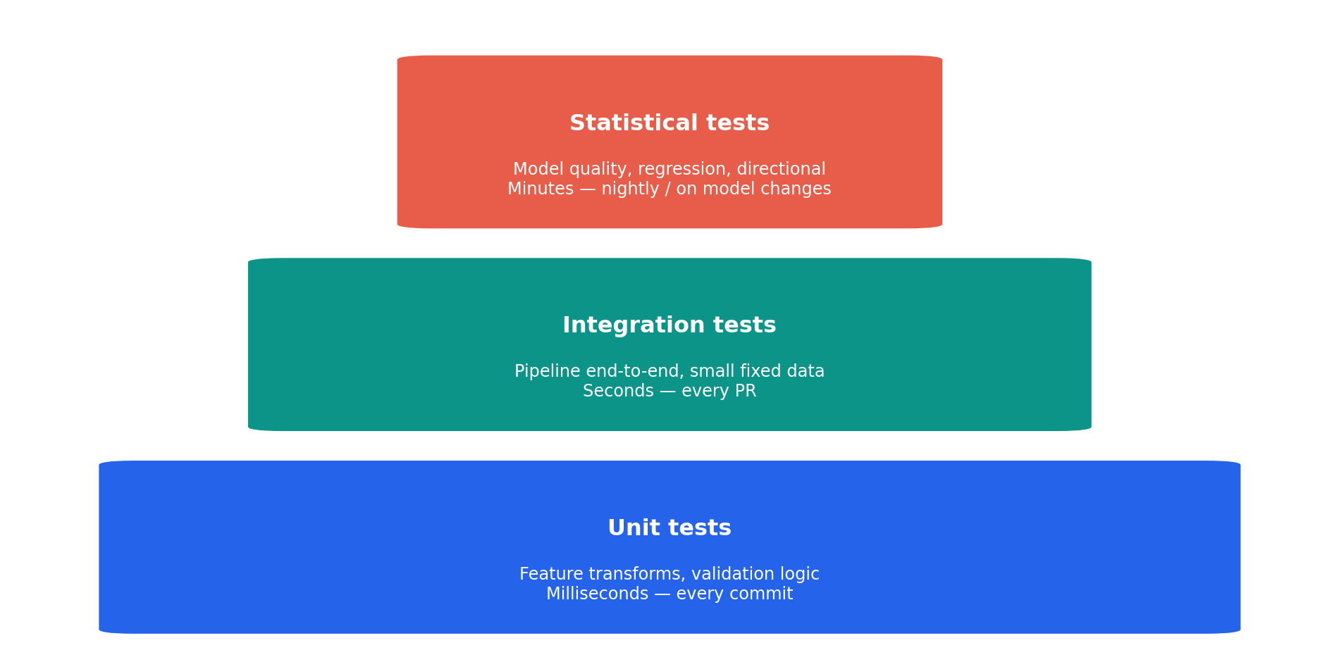
A well-structured test suite for a data science project has three tiers, mirroring the test pyramid from software engineering (Figure 20.2). The pyramid shape (many fast tests at the base, fewer slow tests at the top) applies, though the relative importance differs: in traditional software, a unit test failure is usually more informative than an integration test failure, but in data science, a statistical test that detects model degradation may be the most important test you have.

import matplotlib.pyplot as plt
import matplotlib.patches as patches

fig, ax = plt.subplots(figsize=(10, 5))

tiers = [
    ('Unit tests', 'Feature transforms, validation '
     'logic\nMilliseconds — every commit',
     '#0072B2', 0, 0.9),   # Okabe-Ito blue
    ('Integration tests', 'Pipeline end-to-end, small '
     'fixed data\nSeconds — every PR',
     '#009E73', 1, 0.65),  # Okabe-Ito bluish green
    ('Statistical tests', 'Model quality, regression, '
     'directional\nMinutes — nightly / on model changes',
     '#D55E00', 2, 0.4),   # Okabe-Ito vermilion
]

for label, desc, colour, row, width in tiers:
    left = (1 - width) / 2
    rect = patches.FancyBboxPatch(
        (left, row * 1.1 + 0.05), width, 0.9,
        boxstyle='round,pad=0.03', facecolor=colour,
        edgecolor='white', linewidth=2,
    )
    ax.add_patch(rect)
    ax.text(
        0.5, row * 1.1 + 0.6, label, ha='center',
        va='center', fontsize=12, fontweight='bold',
        color='white',
    )
    ax.text(
        0.5, row * 1.1 + 0.3, desc, ha='center',
        va='center', fontsize=9, color='white',
    )

ax.set_xlim(-0.05, 1.05)
ax.set_ylim(-0.05, 3.4)
ax.axis('off')
fig.patch.set_alpha(0)
ax.patch.set_alpha(0)
plt.tight_layout()
plt.show()

Figure 20.2: The data science test pyramid. Unit tests form the fast, broad base; statistical tests are fewer but catch the most dangerous failures.

In pytest, mark your statistical tests so they can be run separately. The following pytest.ini configuration lets you run pytest -m "not statistical" on every commit (fast) and pytest -m statistical nightly or when model code changes:

[pytest]
markers =
    statistical: tests that involve model training (slow)

A typical project layout mirrors standard application code:

project/
├── src/
│   ├── features.py          # Feature engineering
│   ├── validation.py        # Data validation logic
│   ├── train.py             # Training pipeline
│   └── predict.py           # Prediction service
├── tests/
│   ├── unit/
│   │   ├── test_features.py       # Fast, deterministic
│   │   └── test_validation.py     # Fast, deterministic
│   ├── integration/
│   │   └── test_pipeline.py       # End-to-end, small data
│   ├── statistical/
│   │   ├── test_performance.py    # Cross-validation checks
│   │   └── test_regression.py     # Reference output comparison
│   └── fixtures/
│       ├── sample_data.parquet    # Fixed test datasets
│       └── reference_preds.npy    # Known-good outputs
└── pytest.ini

20.10 Worked example: a tested prediction pipeline

The four patterns above work independently, but they compose. A realistic pipeline needs all of them: deterministic tests for the data transformations, behavioural tests for the model, and leakage tests to catch the silent failures. The incident prediction system below demonstrates all five test types in sequence.

First, the reusable functions: feature engineering and data validation:

def engineer_features(df: pd.DataFrame) -> pd.DataFrame:
    """Transform raw metrics into model features."""
    result = df.copy()
    result['error_rate_log'] = np.log1p(df['error_pct'])
    result['latency_over_threshold'] = (
        df['p99_latency_ms'] > 200
    ).astype(int)
    result['load_x_errors'] = (
        df['request_rate'] * df['error_pct']
    )
    return result


def validate_raw_data(df: pd.DataFrame) -> list[str]:
    """Check raw data before feature engineering."""
    errors = []
    for col in ['error_pct', 'request_rate', 'p99_latency_ms']:
        if col not in df.columns:
            errors.append(f"Missing column: {col}")
        elif df[col].isna().any():
            errors.append(f"Nulls in {col}")
        elif (df[col] < 0).any():
            errors.append(f"Negative values in {col}")
    return errors

Now generate training data and run the deterministic tests: data validation and feature engineering:

rng = np.random.default_rng(42)
n = 1000
raw = pd.DataFrame({
    'error_pct': np.clip(rng.normal(2, 1.5, n), 0, None),
    'request_rate': rng.exponential(100, n),
    'p99_latency_ms': rng.lognormal(4, 0.8, n),
})
log_odds = (
    -3.5
    + 0.4 * raw['error_pct']
    + 0.005 * raw['request_rate']
    + 0.002 * raw['p99_latency_ms']
)
raw['incident'] = rng.binomial(1, expit(log_odds))

# Test 1: Data validation
validation_errors = validate_raw_data(raw)
assert validation_errors == [], (
    f"Validation failed: {validation_errors}"
)
print('Test 1 passed: data validation')

# Test 2: Feature engineering (deterministic)
features = engineer_features(raw)
assert 'error_rate_log' in features.columns
assert 'latency_over_threshold' in features.columns
assert 'load_x_errors' in features.columns
assert features['error_rate_log'].isna().sum() == 0
assert set(
    features['latency_over_threshold'].unique()
).issubset({0, 1})
print('Test 2 passed: feature engineering')

Test 1 passed: data validation
Test 2 passed: feature engineering

Train the model and run the behavioural tests: smoke, minimum performance, and directional:

from sklearn.model_selection import train_test_split, cross_val_score
from sklearn.dummy import DummyClassifier

feature_cols = [
    'error_pct', 'request_rate', 'p99_latency_ms',
    'error_rate_log', 'latency_over_threshold',
    'load_x_errors',
]
X_we = features[feature_cols]
y_we = raw['incident']
X_train, X_test, y_train, y_test = train_test_split(
    X_we, y_we, test_size=0.2, random_state=42
)

we_model = GradientBoostingClassifier(
    n_estimators=100, max_depth=3, random_state=42
)
we_model.fit(X_train, y_train)

# Test 3: Smoke test
preds = we_model.predict(X_test)
probs = we_model.predict_proba(X_test)
assert preds.shape == (len(X_test),)
assert probs.shape == (len(X_test), 2)
assert np.allclose(probs.sum(axis=1), 1.0)
print('Test 3 passed: smoke test')

# Test 4: Minimum performance (vs stratified dummy)
dummy = DummyClassifier(
    strategy='stratified', random_state=42
)
model_auc = cross_val_score(
    we_model, X_we, y_we, cv=5, scoring='roc_auc'
).mean()
dummy_auc = cross_val_score(
    dummy, X_we, y_we, cv=5, scoring='roc_auc'
).mean()
assert model_auc > dummy_auc + 0.05, (
    f"Model AUC ({model_auc:.3f}) doesn't beat "
    f"dummy ({dummy_auc:.3f}) by at least 0.05"
)
print(f"Test 4 passed: performance "
      f"(model AUC={model_auc:.3f} vs dummy={dummy_auc:.3f})")

# Test 5: Directional test
low_error = pd.DataFrame({
    'error_pct': [1.0], 'request_rate': [100.0],
    'p99_latency_ms': [50.0],
    'error_rate_log': [np.log1p(1.0)],
    'latency_over_threshold': [0],
    'load_x_errors': [100.0],
})
high_error = pd.DataFrame({
    'error_pct': [10.0], 'request_rate': [100.0],
    'p99_latency_ms': [50.0],
    'error_rate_log': [np.log1p(10.0)],
    'latency_over_threshold': [0],
    'load_x_errors': [1000.0],
})
p_low = we_model.predict_proba(low_error[feature_cols])[0, 1]
p_high = we_model.predict_proba(
    high_error[feature_cols]
)[0, 1]
assert p_high > p_low, (
    'Higher error rate should increase incident probability'
)
print(f"Test 5 passed: directional "
      f"(low={p_low:.3f}, high={p_high:.3f})")

Test 3 passed: smoke test
Test 4 passed: performance (model AUC=0.613 vs dummy=0.482)
Test 5 passed: directional (low=0.059, high=0.779)

Five tests, five different aspects of correctness. None of them requires knowing the exact model output. Together, they provide strong evidence that the pipeline is working as intended, and they’ll catch most regressions caused by code changes, data shifts, or library upgrades.

20.11 Summary

Testing data science code is testing — the same discipline, the same rigour, the same CI integration you already know. The difference is in what you assert:

1. Test the deterministic parts exactly. Feature engineering, data transforms, and validation logic are ordinary functions. Test them with exact assertions, like any other code.

2. Use tolerances for numerical code. np.testing.assert_allclose with an appropriate tolerance handles floating-point imprecision without making your tests flaky. Set both rtol and atol when values may be near zero.

3. Test model behaviour, not exact outputs. Smoke tests, directional tests, invariance tests, and minimum performance tests together provide strong coverage without requiring you to predict exact model outputs.

4. Test for data leakage explicitly. Temporal leakage and target leakage are the most dangerous data science bugs because they make models look better than they should. Write tests that check for them directly.

5. Validate data at pipeline boundaries. Schema checks, null checks, range checks, and distribution checks catch upstream data problems before they silently corrupt your model’s predictions.

The applied chapters in Part 5 will exercise these patterns on real industry problems — from churn prediction to fraud detection — where the choice of test strategy directly affects business outcomes.

20.12 Exercises

1. Write a validate_prediction_output function that checks model predictions before they’re returned to a consumer. It should verify: (a) no null values, (b) all probabilities are between 0 and 1, (c) probabilities sum to 1 per row (within tolerance), and (d) the predicted class distribution is not suspiciously concentrated (e.g., >99% of predictions are the same class). Write pytest-style tests for each condition, including tests that deliberately trigger each failure.

2. A colleague argues that setting random_state=42 in every test makes the tests pass by coincidence — the model might fail with a different seed. Write a test that trains and evaluates a model across 10 different random seeds and asserts that the accuracy is above a threshold for all of them. What does this test tell you that a single-seed test does not? Where does this approach break down?

3. Build a directional test suite for a churn prediction model. Assume the model takes features tenure_months, monthly_spend, support_tickets_last_30d, and days_since_last_login. Write at least four directional tests, each checking that a plausible change in one feature moves the churn probability in the expected direction. For one of the features, explain a scenario where the expected direction might be wrong.

4. Conceptual: Your team has a model in production with no tests. You’ve been asked to add a test suite retroactively. You can’t write exact-output tests because you don’t know what the “correct” outputs should be — the model is the only source of truth. Describe a strategy for building a test suite from scratch around an existing model. Which types of tests can you add immediately, and which require baseline measurements first?

5. Conceptual: A data scientist on your team says “We don’t need unit tests — we have model evaluation metrics. If the AUC is good, the code is correct.” Write a rebuttal (3–5 sentences). Give at least two concrete examples of bugs that would not be caught by good evaluation metrics but would be caught by the testing patterns described in this chapter.