---
# Content: CC BY-NC-SA 4.0 | Code: MIT - see /LICENSE.md
title: "Data pipelines: ETL and feature stores"
---
{{< include /_common-imports.qmd >}}
## The glue code problem {#sec-pipelines-intro}
A common misconception about machine learning systems is that they're mostly *model* code: the elegant lines where you fit a random forest or tune a gradient boosting classifier. In practice, the model is a small box in the centre of a much larger system. The rest is data pipelines: extracting raw data from sources, transforming it into features the model can consume, loading it into the right place at the right time, and doing all of this reliably, repeatedly, and at scale.
An influential paper on technical debt in ML systems [@sculley2015] called this "glue code": the infrastructure that connects data sources to models and models to decisions. They argued the model itself is only a small fraction of a production ML system — the bulk being data collection, feature extraction, validation, serving infrastructure, and monitoring.
If you've built microservices, this ratio will feel familiar. The business logic in a typical service is a thin layer; the rest is routing, serialisation, error handling, retries, logging, and health checks. Data pipelines are the same pattern applied to data: the statistical transformation is the thin layer, surrounded by engineering that makes it reliable.
This chapter covers the engineering patterns that make data pipelines robust. If @sec-repro-intro was about ensuring your results are reproducible, this chapter is about ensuring the data that feeds those results is correct, consistent, and available when you need it.
## ETL: the part you already know {#sec-etl}
**ETL** — **Extract, Transform, Load** — is the dominant pattern for moving data from source systems into a form suitable for modelling. Each stage maps cleanly onto engineering patterns you already use:
*Extract* reads from an unreliable source (API, database, message queue, file drop). The defensive programming is identical to calling any external service: retries with backoff, schema validation, timeout handling.
*Transform* reshapes the data: joins, filters, type conversions, missing-value handling, derived columns. This is your business logic layer. Pure functions, testable in isolation, deterministic for a given input.
*Load* writes to the destination atomically. Stage, validate, swap — the same pattern as a database transaction or a blue/green deploy.
The mechanics are familiar territory; the data-science-specific bit is what counts as a *valid* transform, and that lives in the next section. Two engineering details *are* worth flagging because they connect to other chapters: **content hashes** on the load output give you the same fingerprinting that @sec-data-repro relies on for reproducibility, and **idempotency** matters more here than in a typical service because pipelines retry routinely and you do not want a partial run leaving the warehouse in a half-loaded state.
::: {.callout-note}
## Engineering Bridge
The mapping is direct: extract is your unreliable upstream call, transform is your business logic, load is your transactional write. The main difference is scale: a microservice processes one request; a pipeline processes a dataset. The principles — idempotency, validation, error handling, atomicity — are unchanged. If your instinct on seeing a flaky external dependency is "wrap it in a retry with backoff and validate the response shape", that instinct ports straight over.
:::
## Feature engineering: the transform layer {#sec-feature-engineering}
In the ETL pattern, the transform step is where data science diverges most from traditional data engineering. A data engineer's transform typically cleans and restructures data: joins, filters, type conversions. A data scientist's transform also creates **features**: derived quantities that encode domain knowledge in a form that models can learn from.
Feature engineering is the process of turning raw data into model inputs. It sounds mechanical, but it's one of the highest-leverage activities in applied data science. A good feature can improve a model more than switching algorithms or tuning hyperparameters. Most of the moves are applied descriptive statistics — the location, spread, and relationship summaries from @sec-descriptive-stats — plus the encoding decisions that translate categorical and ordinal data into numbers a model can consume. The pipeline is industrialised summary statistics, not a separate discipline.
```{python}
#| label: feature-engineering
#| echo: true
rng = np.random.default_rng(42)

# Simulated e-commerce transaction data
n = 2000
transactions = pd.DataFrame({
    'user_id': rng.integers(1, 201, n),
    'timestamp': pd.date_range('2023-06-01', periods=n, freq='37min'),
    'amount': np.round(rng.lognormal(3, 1, n), 2),
    'category': rng.choice(['electronics', 'clothing', 'food', 'books'], n),
})

# Feature engineering: aggregate per-user behaviour
user_features = transactions.groupby('user_id').agg(
    total_spend=('amount', 'sum'),
    avg_transaction=('amount', 'mean'),
    transaction_count=('amount', 'count'),
    unique_categories=('category', 'nunique'),
    max_single_purchase=('amount', 'max'),
).reset_index()

# Derived ratios
user_features['avg_to_max_ratio'] = (
    user_features['avg_transaction'] / user_features['max_single_purchase']
)

print(user_features.describe().round(2))
```
Each of these features encodes a specific hypothesis about user behaviour: users who spend across many categories might behave differently from those who concentrate in one; users whose average transaction is close to their maximum are consistent spenders, while those with a low ratio make occasional large purchases. The model doesn't know these hypotheses; it just sees numbers. The feature engineer's job is to present the numbers in a way that makes the underlying patterns learnable.
::: {.callout-tip}
## Author's Note
There's something genuinely disorienting about feature engineering for an engineer. Our instinct is that the algorithm is the interesting part: the O(n log n) sort, the graph traversal, the clever cache invalidation strategy. Data is just input: the format is a concern of serialisation, not of the algorithm itself. Feature engineering inverts this completely. Two models using identical algorithms on the same raw data can produce wildly different results depending on how the features are constructed. The *representation* is doing the work that we'd normally assign to the algorithm. This feels wrong in the same way that "it depends on how you ask the question" feels wrong to an engineer trained to think that there's a right answer independent of framing. In data science, framing is half the answer.
:::
## The train/serve skew problem {#sec-train-serve-skew}
One of the most insidious bugs in production ML systems is **train/serve skew**: a mismatch between how features are computed during training and how they're computed at serving time. The model learns from one representation of the data but makes predictions on a subtly different one.
This happens more easily than you'd think. During training, you compute features in a batch pipeline using pandas on a static dataset. At serving time, you compute features in real time using a different code path — perhaps a Java service that reimplements the same logic but handles edge cases differently. A rounding difference, a different null-handling strategy, or a time-zone conversion that behaves differently between Python and Java, and your model's predictions degrade silently.
```{python}
#| label: train-serve-skew
#| echo: true
from sklearn.preprocessing import StandardScaler
from sklearn.linear_model import LogisticRegression

rng = np.random.default_rng(42)

# Training: compute features from historical data
train_data = rng.normal(50, 15, (500, 3))
scaler = StandardScaler()
X_train = scaler.fit_transform(train_data)
y_train = (X_train[:, 0] + 0.5 * X_train[:, 1] > 0).astype(int)

model = LogisticRegression(random_state=42)
model.fit(X_train, y_train)

# Serving: a new observation arrives
new_obs = np.array([[65, 40, 55]])

# Correct: use the fitted scaler from training
X_correct = scaler.transform(new_obs)
pred_correct = model.predict_proba(X_correct)[0, 1]

# Skewed: accidentally re-fit the scaler on just the new observation
bad_scaler = StandardScaler()
X_skewed = bad_scaler.fit_transform(new_obs)  # this centres on the single obs!
pred_skewed = model.predict_proba(X_skewed)[0, 1]

print(f'Correct prediction:  {pred_correct:.4f}')
print(f'Skewed prediction:   {pred_skewed:.4f}')
print(f'Difference:          {abs(pred_correct - pred_skewed):.4f}')
```
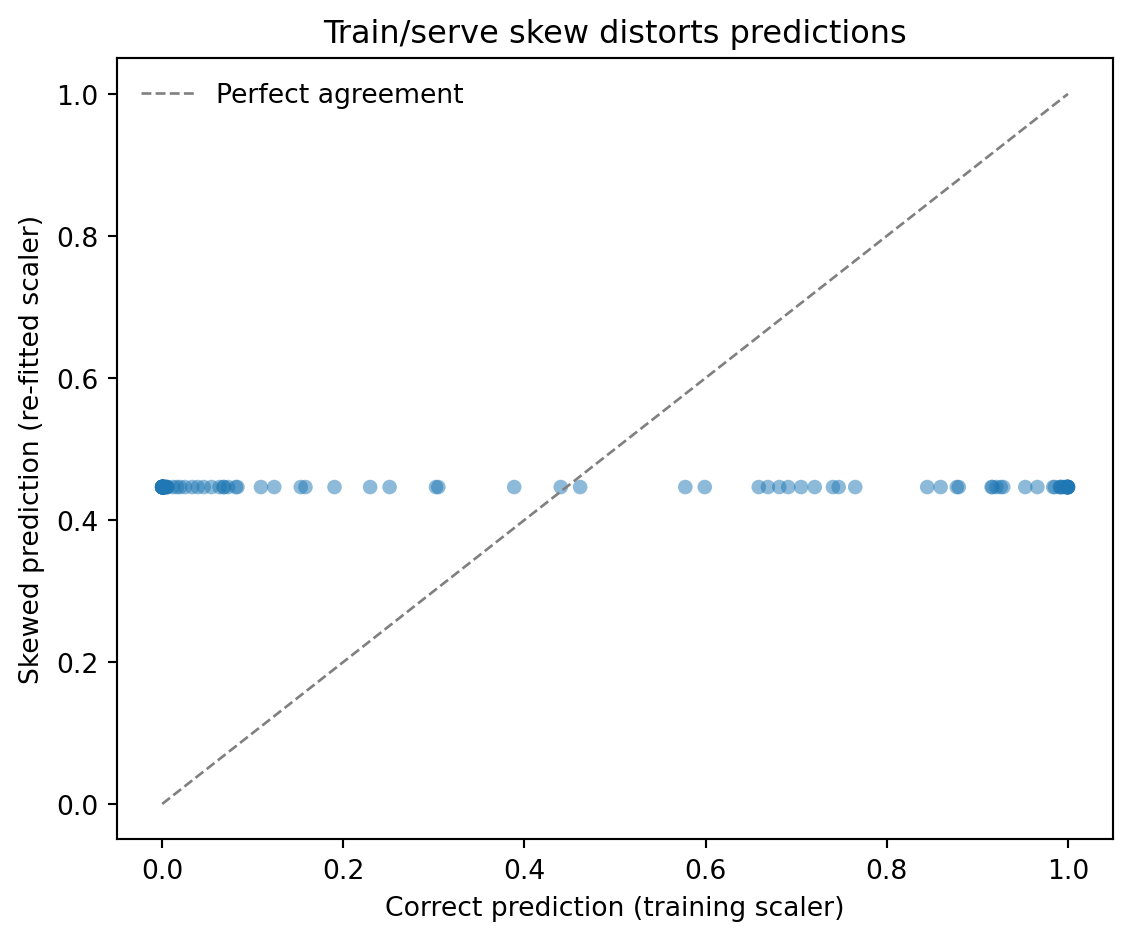
The correct serving path uses the *training* scaler, the one fitted on the training data's mean and standard deviation. The skewed path re-fits a scaler on the single new observation. With only one data point there is no variance to scale by, so scikit-learn guards against the division by zero by setting the scale factor to 1, and mean-centring then maps every feature to exactly zero. The model is handed an all-zeros vector — the origin of standardised space, which corresponds to the training mean — and dutifully returns the prediction it associates with a perfectly average record, regardless of what the observation actually was. No exception is raised; the code runs to completion and returns an answer. It's just the wrong answer.
To see this at scale, we can generate many test observations and compare the correct and skewed predictions for each:
```{python}
#| label: fig-train-serve-skew
#| echo: true
#| fig-cap: "Train/serve skew in action. Each point is a test observation scored
#| two ways: correctly (using the training scaler) and incorrectly (re-fitting
#| a scaler per observation). The skewed predictions collapse to a single value
#| (here ~0.5) because re-fitting the scaler maps every observation to the
#| all-zeros vector — the training mean — destroying all discrimination, while
#| correct predictions span the full probability range."
#| fig-alt: "Scatter plot comparing correct vs skewed predicted probabilities for
#| 100 test observations. Correct predictions spread from 0 to 1 along the
#| x-axis; skewed predictions collapse to a single value near 0.5 on the y-axis,
#| because re-fitting the scaler per observation maps every observation to the
#| training mean, destroying the model's discrimination."
import warnings

test_data = rng.normal(50, 15, (100, 3))
correct_preds = model.predict_proba(scaler.transform(test_data))[:, 1]

skewed_preds = []
for obs in test_data:
    s = StandardScaler()
    with warnings.catch_warnings():
        warnings.simplefilter('ignore')  # suppress divide-by-zero warnings
        x = s.fit_transform(obs.reshape(1, -1))
    skewed_preds.append(model.predict_proba(x)[0, 1])
skewed_preds = np.array(skewed_preds)

fig, ax = plt.subplots(figsize=(6, 5))
fig.patch.set_alpha(0)
ax.patch.set_alpha(0)

ax.scatter(correct_preds, skewed_preds, alpha=0.5, s=30, edgecolors='none', color='#0072B2')
ax.plot([0, 1], [0, 1], '--', color='grey', linewidth=1, label='Perfect agreement')
ax.axhline(0.5, color='#E69F00', linestyle=':', linewidth=1.2, label='Skewed predictions cluster here')
ax.annotate('Re-fitted scaler maps every\nobservation to the training mean',
            xy=(0.8, 0.5), xytext=(0.5, 0.7),
            arrowprops=dict(arrowstyle='->', color='#E69F00'),
            color='#E69F00', fontsize=9)

ax.set_xlabel('Correct prediction (training scaler)')
ax.set_ylabel('Skewed prediction (re-fitted scaler)')
ax.set_title('Re-fitting the scaler at serve time collapses predictions')
ax.legend(frameon=False)
ax.set_xlim(-0.05, 1.05)
ax.set_ylim(-0.05, 1.05)
ax.spines[['top', 'right']].set_visible(False)
plt.tight_layout()
plt.show()
```
### Where skew creeps in {#sec-skew-sources}
The re-fitted scaler is the cleanest demonstration, but it is far from the only path to skew. The cases worth recognising in practice fall into four families.
*Stateful preprocessing drift.* Any transform that learns parameters from data — scalers, normalisers, target encoders, imputers, dimensionality reducers — must be *fitted* once at training time and *applied* unchanged at serving time. Re-fitting in either direction produces silently wrong outputs. The example above is the canonical case; the same trap exists for `OneHotEncoder` (which learns the category vocabulary), `TargetEncoder` (which learns category-to-mean mappings), and `PCA` (which learns the rotation).
*Reimplementation drift.* The training pipeline computes features in pandas; the serving path is a Java microservice that reimplements the same logic for low-latency inference. The reimplementation is "obvious" — until rounding behaviour, time-zone handling, null semantics, or the boundary of a "30-day window" diverges between the two languages. Each individual difference is small; together they degrade predictions in ways that are nearly impossible to attribute to a single cause.
*Time-window misalignment.* A feature defined as "transactions in the last seven days" is unambiguous at training time (the seven days before the label). At serving time it must mean "the seven days before the *prediction request*", which depends on the request's clock, the data's clock, and any latency between an event happening and the feature store catching up. Off-by-a-day errors here are routine and the model has no way to flag them.
*Hidden label leakage in features.* A training feature inadvertently includes information that is only available *after* the prediction would have been made — a status field that gets backfilled, an aggregate that secretly uses future events. Offline metrics look excellent because the leaked information is genuinely predictive; production metrics collapse because the information is not available at serve time. This is the future-leakage cousin of point-in-time correctness, and it is the single most expensive class of skew bug.
### Detecting skew before customers do {#sec-skew-detection}
Three tactics, in roughly increasing engineering cost.
*Logging plus comparison.* Log the feature vector that the model receives at serve time, alongside the prediction. Periodically replay the same inputs through the training-time feature pipeline and compare. Any divergence is skew. This is the equivalent of golden-output regression tests for a service.
*Population statistics monitoring.* For each feature, store summary statistics (mean, standard deviation, percentile distribution) from the training set. In production, compute the same statistics on a rolling window of serve-time features. Significant divergence between training-time and serve-time statistics is either skew or genuine concept drift; both warrant investigation. We will return to monitoring patterns in @sec-model-monitoring.
*Shadow inference.* Deploy the new model to receive production traffic in parallel with the existing model, but discard its predictions. Compare the shadow model's predictions to a periodically-rerun training-time evaluation on the same inputs. Persistent gaps point at skew before the new model ever influences decisions.
The mitigations are mostly variations on a single principle: **make the same code compute features in both paths**. Serialise fitted preprocessors with the model (use `joblib.dump` so the scaler ships with the model artefact and cannot be silently re-fitted). Push feature computation into a shared library that both training and serving import. When that is impractical — typically because of latency or language constraints — invest in the comparison tooling above so divergence is detected automatically rather than by the eventual customer complaint.
::: {.callout-note}
## Engineering Bridge
Train/serve skew is the data science equivalent of **dev/prod parity**, one of the twelve-factor app principles. In web development you learn — usually the hard way — that if dev uses SQLite and production uses PostgreSQL, you'll discover bugs only in production. Feature computation is the same problem at a different layer: training and serving are two environments computing the same logical thing, and any divergence between them shows up as model degradation rather than as a stack trace. The fix is also the same: minimise the gap. Treat the fitted scaler as part of the model artefact, not as throwaway scaffolding; ship a single feature library that both pipelines import; and where you cannot share code, automate the comparison so divergence cannot drift unchecked.
:::
## Feature stores: the shared library of features {#sec-feature-stores}
A **feature store** is infrastructure that solves two problems at once: it provides a single, shared repository of feature definitions (eliminating duplicate feature engineering across teams), and it serves the same features consistently for both training and inference (eliminating train/serve skew).
Instead of each model reimplementing "days since last purchase" or "average transaction amount over 30 days," these features are defined once, computed by a shared pipeline, and stored in a system that serves them to any model that needs them. Training reads historical features as of the time each training example occurred (point-in-time correctness). Serving reads the latest feature values for real-time predictions.
Feature stores typically have two storage layers. The **offline store** — a data warehouse or file system — holds historical features used in training, stored as a large columnar dataset keyed by entity ID and timestamp. The **online store** — a low-latency key-value store like Redis or DynamoDB — holds the latest feature values used in real-time serving. A synchronisation process keeps the online store up to date as the offline store is refreshed.
```{python}
#| label: feature-store-concept
#| echo: true
rng = np.random.default_rng(42)

# Simulate a feature store's offline layer: historical features keyed by
# (user_id, event_timestamp)
n_users = 50
n_snapshots = 12  # monthly snapshots

records = []
for user_id in range(1, n_users + 1):
    base_spend = rng.exponential(200)
    for month in range(n_snapshots):
        records.append({
            'user_id': user_id,
            'snapshot_date': pd.Timestamp('2023-01-01') + pd.DateOffset(months=month),
            'total_spend_30d': round(base_spend * rng.uniform(0.5, 1.5), 2),
            'transaction_count_30d': int(rng.poisson(8)),
            'days_since_last_purchase': int(rng.exponential(5)),
        })

offline_store = pd.DataFrame(records)
print(f'Offline store: {offline_store.shape[0]} rows '
      f'({n_users} users x {n_snapshots} snapshots)')
print(f'Columns: {list(offline_store.columns)}')
print()

# Point-in-time lookup: get features as they were on a specific date
def get_features_at(store: pd.DataFrame, user_id: int,
                    as_of: pd.Timestamp) -> pd.Series:
    """Retrieve features for a user as of a given date."""
    mask = (store['user_id'] == user_id) & (store['snapshot_date'] <= as_of)
    if mask.sum() == 0:
        return pd.Series(dtype=float)
    return store.loc[mask].sort_values('snapshot_date').iloc[-1]

# Training: get features as of training label date (avoids future leakage)
train_features = get_features_at(offline_store, user_id=1,
                                  as_of=pd.Timestamp('2023-06-15'))
print('Training features for user 1 as of 2023-06-15:')
print(train_features[['total_spend_30d', 'transaction_count_30d',
                       'days_since_last_purchase']].to_string())
```
The `get_features_at` function illustrates the critical concept of **point-in-time correctness**. When building training data, you must retrieve features as they existed *at the time the label was observed*, not as they exist today. Using today's features to predict yesterday's outcome is data leakage: the model sees information from the future during training, learns to rely on it, and then fails in production where that information isn't available. The operational symptom is characteristically deceptive: offline evaluation metrics look excellent, but the model underperforms as soon as it is deployed. The gap between trained accuracy and live accuracy is the fingerprint of future leakage.
::: {.callout-note}
## Engineering Bridge
A feature store is to ML features what a package registry (npm, PyPI, Maven) is to code libraries. Without a registry, every team copies and modifies shared code independently, leading to inconsistent behaviour and duplicated maintenance. A package registry provides a single source of truth with versioning and dependency management. A feature store does the same for computed features: it provides a canonical definition, historical versioning, and consistent access for both training (batch reads of historical data) and serving (real-time reads of current values). The parallel even extends to the governance problem: just as a package registry lets you audit who depends on a library before changing its API, a feature store lets you audit which models depend on a feature before changing its computation logic.
:::
## Data validation: catching problems early {#sec-data-validation}
The most expensive bugs in data pipelines are the ones that don't crash. A malformed API response that gets silently ingested, a join that drops rows due to a key mismatch, a feature column that drifts to all zeros after an upstream schema change — these produce valid-looking data that quietly degrade your model's predictions.
Data validation is the practice of asserting expectations about your data at each stage of the pipeline, the same way you'd add assertions and contract tests to a service boundary.
```{python}
#| label: data-validation
#| echo: true
def validate_features(df: pd.DataFrame) -> list[str]:
    """Validate a feature DataFrame against expected contracts."""
    errors = []

    # Schema checks
    required_cols = {'user_id', 'total_spend', 'transaction_count',
                     'unique_categories'}
    missing = required_cols - set(df.columns)
    if missing:
        errors.append(f'Missing columns: {missing}')

    # Null checks
    null_pct = df.isnull().mean()
    high_null_cols = null_pct[null_pct > 0.05].index.tolist()
    if high_null_cols:
        errors.append(f'Columns exceed 5% null threshold: {high_null_cols}')

    # Range checks
    if 'total_spend' in df.columns and (df['total_spend'] < 0).any():
        errors.append('Negative values in total_spend')

    if 'transaction_count' in df.columns and (df['transaction_count'] < 0).any():
        errors.append('Negative values in transaction_count')

    # Distribution checks (detect drift)
    if 'total_spend' in df.columns:
        median_spend = df['total_spend'].median()
        if median_spend < 1 or median_spend > 10_000:
            errors.append(f'Suspicious median total_spend: {median_spend:.2f}')

    # Completeness check
    if len(df) < 100:
        errors.append(f'Fewer than 100 rows ({len(df)}) — possible extraction failure')

    return errors

# Test with clean data
rng = np.random.default_rng(42)
good_data = pd.DataFrame({
    'user_id': range(500),
    'total_spend': rng.exponential(200, 500),
    'transaction_count': rng.poisson(10, 500),
    'unique_categories': rng.integers(1, 6, 500),
})

errors = validate_features(good_data)
print(f'Clean data validation: {"PASSED" if not errors else errors}')

# Test with problematic data
bad_data = good_data.copy()
bad_data.loc[:40, 'total_spend'] = np.nan  # >5% nulls
bad_data.loc[100:105, 'transaction_count'] = -1  # negative counts

errors = validate_features(bad_data)
print(f'Bad data validation:   {errors}')
```
The validation function checks four categories of expectation: **schema** (are the right columns present?), **nulls** (is data completeness within tolerance?), **ranges** (are values physically plausible?), and **distributions** (has the data drifted from expected patterns?). In production, these checks run at every pipeline stage: after extraction, after each transform, and before load. If any check fails, the pipeline halts and alerts the team rather than silently writing bad data.
::: {.callout-tip}
## Author's Note
Data validation feels like a "nice to have", something you add after the pipeline is working. But pipelines fail silently far more often than they fail loudly. A column that changes from British date format (DD/MM/YYYY) to American format (MM/DD/YYYY) will parse without error (e.g., 1 March becomes 3 January) and the model will retrain on quietly wrong features. The accuracy drop will be subtle, delayed, and extremely hard to diagnose after the fact. A simple validation check at the pipeline boundary catches these problems in seconds. The instinct should be: write the validation *before* the transform, not after.
:::
## Orchestrating pipeline stages {#sec-orchestration}
A real-world feature pipeline is a DAG of dependent stages: extraction, transform, validation, load — each gated on the previous succeeding. **Airflow** is the established standard; **Prefect** is a more Pythonic alternative; **Dagster** emphasises typed data contracts between stages. All three give you the same primitives a CI/CD system gives you for code: task graphs, retries, scheduling, and alerting.
```{python}
#| label: airflow-dag-concept
#| eval: false
#| echo: true
# In any of these tools, the dependency syntax is essentially the same:
extract >> transform >> validate >> load
```
The `>>` operator defines execution order. `validate` does not run until `transform` succeeds; if `validate` fails, `load` never executes and bad data never reaches the feature store. The orchestrator layers on scheduling (run daily at 02:00), retries (re-run `extract` three times with exponential backoff), and alerting (page on-call if the pipeline has not succeeded by 06:00). This is exactly the GitHub Actions / GitLab CI mental model applied to data instead of code.
## A worked example: end-to-end feature pipeline {#sec-pipeline-worked-example}
The following example brings together the concepts from this chapter: extraction, validation, feature engineering, and reproducible output. We'll build a feature pipeline for the service metrics scenario from @sec-repro-worked-example and demonstrate how each stage validates its outputs.
```{python}
#| label: pipeline-worked-example
#| echo: true
import hashlib
import io
from datetime import datetime, timezone

# ---- Stage 1: Extract ----
rng = np.random.default_rng(42)
n = 1500

p50_latency = rng.lognormal(3, 0.5, n)

raw_metrics = pd.DataFrame({
    'service_id': rng.choice(['api-gateway', 'auth-service', 'payment-svc',
                               'search-api', 'user-svc'], n),
    'timestamp': pd.date_range('2023-01-01', periods=n, freq='6h'),
    'request_rate': rng.exponential(500, n),
    'error_count': rng.poisson(5, n),
    'p50_latency_ms': p50_latency,
    'p99_latency_ms': p50_latency + rng.exponential(30, n),  # p99 >= p50 by definition
    'cpu_pct': np.clip(rng.normal(45, 20, n), 0, 100),
})

# Introduce realistic messiness
raw_metrics.loc[rng.choice(n, 20, replace=False), 'error_count'] = np.nan
raw_metrics.loc[rng.choice(n, 10, replace=False), 'cpu_pct'] = -1  # sensor glitch

print(f'Extracted: {raw_metrics.shape[0]} rows from 5 services')
print(f'  Nulls: {raw_metrics.isna().sum().sum()}, '
      f'Invalid CPU: {(raw_metrics["cpu_pct"] < 0).sum()}')
```
The raw extract has the usual problems: null error counts (perhaps the monitoring agent was down during those intervals) and negative CPU readings from a sensor glitch. Before transforming the extracted data, we validate the extraction to catch catastrophic failures early: a truncated extract or a missing column would waste everything downstream.
```{python}
#| label: pipeline-validate-extract
#| echo: true
# ---- Stage 2: Validate extraction ----
def validate_extraction(df: pd.DataFrame) -> list[str]:
    """Gate check after extraction."""
    errors = []
    required = {'service_id', 'timestamp', 'request_rate', 'error_count',
                'p50_latency_ms', 'p99_latency_ms', 'cpu_pct'}
    missing = required - set(df.columns)
    if missing:
        errors.append(f'Missing columns: {missing}')
    if len(df) < 100:
        errors.append(f'Too few rows: {len(df)}')
    if df['timestamp'].nunique() < 10:
        errors.append('Suspiciously few unique timestamps')
    return errors

extract_errors = validate_extraction(raw_metrics)
print(f'Extraction validation: {"PASSED" if not extract_errors else extract_errors}')
```
With the extraction validated, the transform stage cleans the data and engineers features. Notice that we fill missing values using per-service medians rather than a global median; the error rate for `payment-svc` is likely on a different scale from `search-api`, so a global fill would blur meaningful differences between services.
```{python}
#| label: pipeline-transform
#| echo: true
# ---- Stage 3: Transform — clean and engineer features ----
def transform_service_metrics(df: pd.DataFrame) -> pd.DataFrame:
    """Clean raw metrics and compute service-level features."""
    clean = df.copy()

    # Fix invalid values
    clean.loc[clean['cpu_pct'] < 0, 'cpu_pct'] = np.nan

    # Fill missing values with per-service medians
    for col in ['error_count', 'cpu_pct']:
        clean[col] = clean.groupby('service_id')[col].transform(
            lambda s: s.fillna(s.median())
        )

    # Derive features
    clean['error_rate'] = clean['error_count'] / clean['request_rate'].clip(lower=1)
    clean['latency_ratio'] = clean['p99_latency_ms'] / clean['p50_latency_ms'].clip(lower=1)
    clean['is_high_cpu'] = (clean['cpu_pct'] > 80).astype(int)

    # Time-based features
    clean['hour'] = clean['timestamp'].dt.hour
    clean['is_business_hours'] = clean['hour'].between(9, 17).astype(int)

    return clean

features = transform_service_metrics(raw_metrics)
print(f'Transformed: {features.shape[0]} rows, {features.shape[1]} columns')
print('  New features: error_rate, latency_ratio, is_high_cpu, hour, is_business_hours')
print(f'  Remaining nulls: {features.isna().sum().sum()}')
```
The transform has cleaned the data and produced five new features. Visualising their distributions gives us a quick sanity check, and establishes a baseline that future pipeline runs can be compared against to detect drift.
```{python}
#| label: fig-feature-distributions
#| echo: true
#| fig-cap: "Distributions of the three continuous features produced by the
#| transform stage: error rate (right-skewed, concentrated near zero),
#| latency ratio (right-skewed, centred around 2), and CPU utilisation
#| (roughly normal, centred around 45%). These baselines are what a
#| distribution drift check would compare against on future pipeline runs."
#| fig-alt: "Three histograms displaying feature distributions from the
#| transform stage. The first histogram shows error rate: heavily
#| right-skewed with most values near zero. The second shows latency ratio
#| (p99 divided by p50): right-skewed, concentrated between 1 and 4. The
#| third shows CPU utilisation percentage: approximately normal, centred
#| near 45. Each histogram has an orange dashed vertical line marking the
#| median."
fig, axes = plt.subplots(1, 3, figsize=(10, 3.5))
fig.patch.set_alpha(0)

feat_cols = ['error_rate', 'latency_ratio', 'cpu_pct']
titles = ['Error rate (errors / requests)', 'Latency ratio (p99 / p50)', 'CPU utilisation (%)']
xlabels = ['Error rate', 'Latency ratio', 'CPU (%)']

for ax, col, title, xlabel in zip(axes, feat_cols, titles, xlabels):
    ax.patch.set_alpha(0)
    ax.hist(features[col].dropna(), bins=40, color='#0072B2',
            edgecolor='white', linewidth=0.5)
    ax.set_xlabel(xlabel)
    ax.set_ylabel('Count')
    ax.set_title(title)
    ax.axvline(features[col].median(), color='#E69F00', linestyle='--', linewidth=1,
               label=f'Median: {features[col].median():.2f}')
    ax.legend(fontsize=8, frameon=False)
    ax.spines[['top', 'right']].set_visible(False)

plt.tight_layout()
plt.show()
```
Now we validate the output; this is the gate between transform and load, and it's where we check invariants that should hold after a correct transformation. If any check fails, the pipeline halts rather than writing bad features to the store.
```{python}
#| label: pipeline-validate-transform
#| echo: true
# ---- Stage 4: Validate transform output ----
def validate_features_pipeline(df: pd.DataFrame) -> list[str]:
    """Gate check after feature engineering."""
    errors = []

    # No nulls should remain after transform
    null_cols = df.columns[df.isna().any()].tolist()
    if null_cols:
        errors.append(f'Unexpected nulls in: {null_cols}')

    # Derived features should be non-negative
    for col in ['error_rate', 'latency_ratio']:
        if col in df.columns and (df[col] < 0).any():
            errors.append(f'Negative values in {col}')

    # Latency ratio should be >= 1 (p99 >= p50 by definition). This cannot fire
    # on the current data, where p99 is constructed as p50 + a non-negative term;
    # it is a defensive guard against upstream changes that break that invariant.
    if 'latency_ratio' in df.columns:
        below_one = (df['latency_ratio'] < 1.0).mean()
        if below_one > 0.05:
            errors.append(f'Latency ratio < 1 for {below_one:.1%} of rows')

    return errors

transform_errors = validate_features_pipeline(features)
print(f'Transform validation: {"PASSED" if not transform_errors else transform_errors}')
```
With both validation gates passed, we can safely load the features. The load step writes the data and produces a manifest: a summary record that captures the pipeline's provenance: row counts, a content hash, and the results of every validation check.
```{python}
#| label: pipeline-load
#| echo: true
# ---- Stage 5: Load with provenance ----
buf = io.BytesIO()
features.to_parquet(buf, index=False)
content_hash = hashlib.sha256(buf.getvalue()).hexdigest()[:16]

manifest = {
    'pipeline': 'service_features',
    'timestamp': datetime.now(timezone.utc).isoformat(),
    'input_rows': len(raw_metrics),
    'output_rows': len(features),
    'output_columns': len(features.columns),
    'content_hash': content_hash,
    'validation': {
        'extract': 'PASSED' if not extract_errors else extract_errors,
        'transform': 'PASSED' if not transform_errors else transform_errors,
    },
}

print('Pipeline manifest:')
for key, value in manifest.items():
    print(f'  {key}: {value}')
```
Each stage validates its output before the next stage begins. The final manifest records the full provenance: how many rows entered, how many survived, what the output hash is, and whether every validation gate passed. This is the data pipeline equivalent of a CI build report: a complete record of what happened, in what order, with what results.
## Summary {#sec-pipelines-summary}
1. **Data pipelines are the majority of ML code.** The model is a small component; the infrastructure that extracts, transforms, validates, and serves data is where most engineering effort goes.
2. **ETL is a pattern, not a technology.** Extract handles unreliable sources with defensive programming. Transform encodes domain knowledge as features. Load writes results atomically with content hashes for verification.
3. **Train/serve skew is a silent killer.** Use the same code path for computing features in training and in serving. Feature stores formalise this by providing a single source of truth for feature definitions and values.
4. **Validate data at every pipeline boundary.** Check schemas, null rates, value ranges, and distributions after each stage. A pipeline that halts on bad data is better than one that silently produces bad predictions.
5. **Orchestrate with DAGs.** Express pipeline dependencies explicitly using tools like Airflow, Prefect, or DVC. This gives you automatic retries, dependency tracking, and the confidence that no stage runs before its inputs are ready and validated.
## Exercises {#sec-pipelines-exercises}
1. Extend the `validate_features` function from @sec-data-validation to include a **distribution drift check**: compare the mean and standard deviation of each numerical column against reference statistics (provided as a dictionary), and flag any column where the mean has shifted by more than 2 standard deviations. Test it by creating a "drifted" dataset where one feature's mean has shifted.
2. Write a feature engineering function that takes the raw transaction data from @sec-feature-engineering and computes **time-windowed features**: for each user, calculate total spend and transaction count over the last 7 days, 30 days, and 90 days relative to a given reference date. Discuss why the reference date matters for avoiding data leakage.
3. Demonstrate the train/serve skew problem with a `StandardScaler`: train a logistic regression model using `fit_transform` on the training set, then show that (a) using `transform` with the training scaler produces correct serving predictions, and (b) calling `fit_transform` on each new observation individually produces wrong predictions. Measure the average prediction error between the two approaches.
4. **Conceptual:** Your company has 15 ML models in production, and 8 of them use a feature called "customer lifetime value" (CLV). Each model team computes CLV slightly differently — different time windows, different revenue definitions, different null handling. A colleague proposes building a feature store to standardise this. What are the benefits? What are the risks? How would you handle the transition without breaking existing models?
5. **Conceptual:** A junior data scientist argues that data validation is unnecessary because "the model will just learn to handle bad data." In what sense are they wrong? In what narrow sense might they have a point? What's the strongest argument for validation that goes beyond model accuracy?
 {#fig-train-serve-skew width=567 height=470 fig-alt=’ Scatter plot comparing correct vs skewed predicted probabilities for
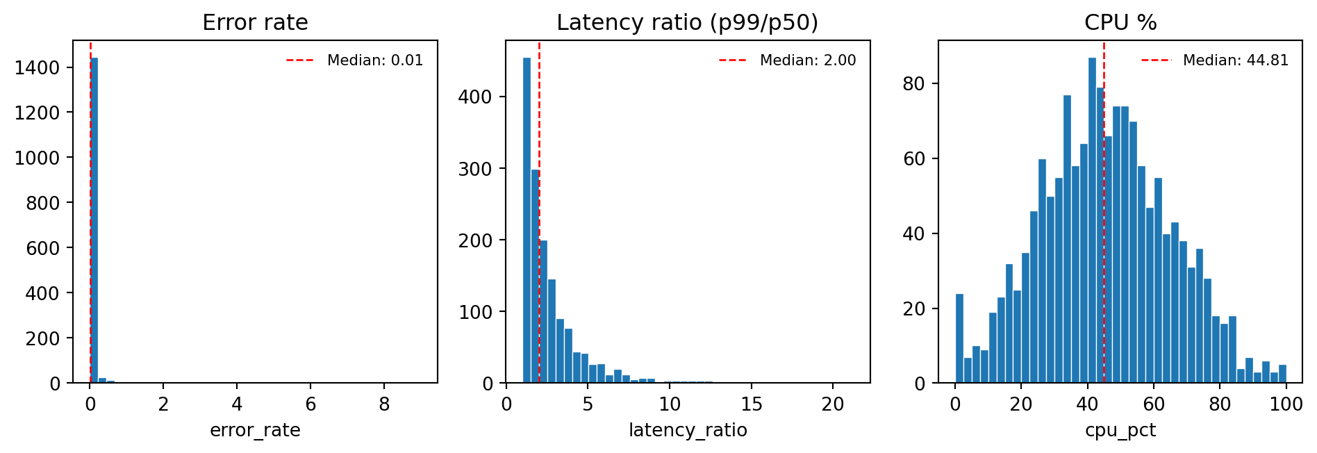 {#fig-feature-distributions width=952 height=326 fig-alt=’ Three histograms displaying feature distributions from the