---
# Content: CC BY-NC-SA 4.0 | Code: MIT - see /LICENSE.md
title: "Model deployment and MLOps"
---
{{< include /_common-imports.qmd >}}
## The model that never left the notebook {#sec-mlops-intro}
You've trained a model. It scores well on the test set, the stakeholders are impressed, and the pull request for the training pipeline has been approved. Now what?
In software engineering, the answer is obvious: deploy it. You've done it hundreds of times: merge to `main`, CI runs, the artefact ships to production. But deploying a model is not like deploying a web service. A web service is deterministic code that either works or crashes. A model is a statistical artefact whose behaviour degrades silently. It can return HTTP 200 with increasingly wrong predictions and nobody notices until a business metric drops weeks later.
This gap between "the model works on my laptop" and "the model reliably serves predictions in production" is what **MLOps** addresses. MLOps borrows from DevOps the idea that the lifecycle doesn't end at development; it includes deployment, monitoring, and continuous improvement. If @sec-repro-intro was about making results reproducible and @sec-pipelines-intro was about making data reliable, this chapter is about making models *operational*.
The good news: most of the infrastructure patterns come directly from software engineering. The complication: models introduce new failure modes that traditional monitoring won't catch.
## Serialising a model {#sec-model-serialisation}
Before a model can be deployed, it must be saved to a file (**serialised**) so that a separate serving process can load and use it without retraining. This is analogous to compiling source code into a binary: the training script is the source, the serialised model is the artefact.
scikit-learn models are Python objects, and the standard serialisation tool for Python objects is `pickle`. The `joblib` library (bundled with scikit-learn) provides a more efficient variant for objects containing large NumPy arrays:
```{python}
#| label: model-serialisation
#| echo: true
from scipy.special import expit  # logistic sigmoid: 1 / (1 + exp(-x))
from sklearn.ensemble import GradientBoostingClassifier
from sklearn.model_selection import train_test_split
from sklearn.preprocessing import StandardScaler
from sklearn.pipeline import Pipeline
import joblib
import io

rng = np.random.default_rng(42)

# Generate synthetic data — SRE incident prediction scenario
n = 800
X = np.column_stack([
    rng.exponential(100, n),       # request_rate
    np.clip(rng.normal(2, 1.5, n), 0, None),  # error_pct
    rng.lognormal(4, 0.8, n),      # p99_latency_ms
    rng.integers(0, 24, n),        # deploy_hour
    rng.binomial(1, 2/7, n),       # is_weekend
])
log_odds = -1.8 + 0.005 * X[:, 0] + 0.8 * X[:, 1] + 0.002 * X[:, 2] + 0.3 * X[:, 4]
y = rng.binomial(1, expit(log_odds))
# Note: this data-generating process produces roughly 62% positive-class examples
# (incidents). Real incident data is often more imbalanced; the imbalance here
# simplifies the worked example but means the dummy-classifier baseline is high.

X_train, X_test, y_train, y_test = train_test_split(
    X, y, test_size=0.2, random_state=42
)

# Package preprocessing + model into a single pipeline
pipeline = Pipeline([
    ('scaler', StandardScaler()),
    ('model', GradientBoostingClassifier(
        n_estimators=150, max_depth=4, learning_rate=0.1, random_state=42
    )),
])
pipeline.fit(X_train, y_train)

# Serialise the entire pipeline — scaler and model together
buf = io.BytesIO()
joblib.dump(pipeline, buf)
model_size_kb = buf.tell() / 1024

print(f"Pipeline test accuracy: {pipeline.score(X_test, y_test):.4f}")
print(f"Serialised size: {model_size_kb:.1f} KB")

# Deserialise and verify identical predictions
buf.seek(0)
loaded = joblib.load(buf)
assert np.array_equal(pipeline.predict(X_test), loaded.predict(X_test))
print('Loaded model predictions match original: True')
```
The critical detail is that we serialise the entire `Pipeline`, scaler and model together. This is the solution to the train/serve skew problem from @sec-train-serve-skew: the serving process loads a single artefact that contains both the preprocessing logic (with its fitted parameters) and the model. There is no opportunity for the scaler to be re-fitted or for a different normalisation path to be used.
::: {.callout-note}
## Engineering Bridge
A serialised pipeline is superficially similar to a **fat JAR**: both bundle everything needed to run into a single file. But the deeper point is different. A fat JAR bundles *code and dependencies*, things that were always there, just in separate locations. A serialised pipeline bundles *learned state*: the scaler's fitted mean and variance, the model's learned tree structure or weight matrix, calibration parameters. None of this existed before training; it was derived from data. That makes the artefact more fragile than a fat JAR in a specific way: the same code with different training data produces a different artefact, and there is no equivalent of a "compile error" when the state is wrong.
The practical consequence is that you must treat the artefact as immutable and content-addressed, the same way you'd treat a container image layer. A model registry provides this discipline. And like a fat JAR, the serialised pipeline carries no runtime environment: the serving process must have the correct scikit-learn and NumPy versions installed, because a version mismatch can cause silent prediction differences rather than import errors. Container images (as discussed in @sec-env-repro) solve this for serving too.
:::
## Model registries: version control for artefacts {#sec-model-registry}
A serialised model file on someone's laptop is not a deployment strategy. Teams need a central place to store model artefacts, track their lineage, and manage which version is currently serving in production. This is what a **model registry** provides.
A model registry is to models what a container registry (Docker Hub, ECR, GCR) is to Docker images: a versioned repository of deployable artefacts with metadata. Each entry records the model version, the training data hash, the evaluation metrics, and the deployment status (staging, production, archived).
MLflow provides the most widely adopted open-source model registry. Each model version moves from initial logging during an experiment run, to registration under a name, to promotion by attaching an **alias** such as `staging` or `production`. (Earlier MLflow releases promoted versions through named *stages*; stages were deprecated in MLflow 2.9 in favour of aliases, which are more flexible — you can define whatever alias names your deployment process needs.) The following illustrates the workflow (this is conceptual; it requires a running MLflow server):
```python
# Conceptual — requires a running MLflow tracking server
import mlflow

# During training: log the model
with mlflow.start_run():
    mlflow.sklearn.log_model(pipeline, 'incident-predictor')
    mlflow.log_metric('test_accuracy', 0.70)
    mlflow.log_param('data_hash', 'a1b2c3d4e5f67890')

# After review: register and promote
model_uri = 'runs:/<run-id>/incident-predictor'
mlflow.register_model(model_uri, 'incident-predictor')

# Promote to production (after staging validation) by attaching an alias
client = mlflow.tracking.MlflowClient()
client.set_registered_model_alias(
    name='incident-predictor', alias='production', version=3
)
# Downstream, load whatever version currently holds the alias:
# mlflow.sklearn.load_model('models:/incident-predictor@production')
```
The registry gives you an audit trail: which model is serving, who promoted it, when, and against what data it was validated. When a model misbehaves in production, you can trace back to the exact training run, data version, and configuration that produced it, the same provenance chain we built in @sec-experiment-tracking, but now extended through deployment. It also enables **rollback**: reverting to a previous model version means re-promoting an earlier registry entry and redeploying, which should be a single command rather than a three-hour scramble at 2am.
## Deployment patterns {#sec-deployment-patterns}
How a model serves predictions depends on the latency requirements and the volume of requests. There are two fundamental patterns, and most production systems use one or both.
**Batch prediction** computes predictions for a large set of inputs on a schedule: nightly, hourly, or triggered by a pipeline completion. The results are written to a database or file, and downstream systems read from the precomputed table. This is the simplest deployment pattern and covers many use cases: churn scores, recommendation lists, risk ratings, and any prediction that doesn't need to reflect the very latest data.
**Real-time prediction** serves predictions on demand, one request at a time, with latency constraints (typically under 100 ms). This is the pattern for fraud detection at the point of transaction, dynamic pricing, search ranking, and any context where the prediction must reflect the current input. The model runs behind an API endpoint, receives a feature vector, and returns a prediction.
```{python}
#| label: deployment-patterns
#| echo: true
import time

# ---- Batch prediction ----
# Score a full dataset in one call — high throughput, high latency per batch
batch_inputs = X_test
start = time.perf_counter()
batch_predictions = pipeline.predict_proba(batch_inputs)[:, 1]
batch_time = time.perf_counter() - start

# ---- Real-time prediction ----
# Score one observation at a time — low latency per request
single_input = X_test[0:1]
latencies = []
for _ in range(100):
    start = time.perf_counter()
    pipeline.predict_proba(single_input)
    latencies.append((time.perf_counter() - start) * 1000)  # ms

latencies = np.array(latencies)

# Note: these measure pure in-process inference time. In production,
# serving latency also includes network overhead, serialisation, input
# validation, and feature lookups — typically 10–100× higher.
print('Batch prediction:')
print(f"  {len(batch_inputs)} observations in {batch_time*1000:.1f} ms")
print(f"  Throughput: {len(batch_inputs)/batch_time:.0f} obs/sec")
print(f"\nReal-time inference (single observation, in-process):")
print(f"  p50 latency: {np.percentile(latencies, 50):.2f} ms")
print(f"  p99 latency: {np.percentile(latencies, 99):.2f} ms")
```
::: {.callout-note}
## Engineering Bridge
Batch vs real-time prediction maps directly onto **asynchronous vs synchronous processing** in backend systems. Batch prediction is a job queue: compute results ahead of time and serve them from a cache (a database table). Real-time prediction is a synchronous API call: the client blocks until the model returns. The engineering trade-offs are identical: batch is simpler, cheaper, and more fault-tolerant; real-time is more responsive but requires careful attention to latency, scaling, and availability. Most production ML systems start with batch and add real-time only where the use case demands it, exactly as you'd start with a cron job and add a real-time API only when polling isn't fast enough.
:::
## Serving a model behind an API {#sec-model-serving}
For real-time prediction, the model needs an HTTP endpoint. The simplest approach wraps the model in a lightweight web framework (Flask, FastAPI, or similar). In production, dedicated model serving tools (MLflow's built-in server, TensorFlow Serving, or Seldon Core) handle scaling, versioning, and health checks, but the core pattern is the same: load the artefact at startup, expose a predict endpoint, validate inputs, return predictions. The following illustrates the pattern (this is conceptual; it requires Flask to be installed):
```python
# Conceptual — requires Flask; illustrates the serving pattern
from flask import Flask, request, jsonify
import joblib
import numpy as np

app = Flask(__name__)
pipeline = joblib.load('models/incident-predictor-v3.joblib')

FEATURE_NAMES = [
    'request_rate', 'error_pct', 'p99_latency_ms',
    'deploy_hour', 'is_weekend',
]

@app.route('/predict', methods=['POST'])
def predict():
    data = request.get_json()

    # Validate input schema (in production, use a schema validation
    # library like Pydantic for type and range checking too)
    missing = [f for f in FEATURE_NAMES if f not in data]
    if missing:
        return jsonify({'error': f"Missing features: {missing}"}), 400

    features = np.array([[data[f] for f in FEATURE_NAMES]])
    probability = float(pipeline.predict_proba(features)[0, 1])

    return jsonify({
        'incident_probability': round(probability, 4),
        'model_version': 'v3',
    })
```
The serving code is deliberately minimal: a thin wrapper around the serialised pipeline. The preprocessing (scaling) happens inside the pipeline, the prediction happens inside the model, and the endpoint handles only HTTP plumbing. This is by design: the less logic in the serving layer, the less opportunity for train/serve skew.
## Safe deployment strategies {#sec-safe-deployment}
Deploying a new model version to production is a risky operation. Unlike deploying a new version of a web service — where bugs typically manifest as errors or crashes — a bad model manifests as *wrong answers that look correct*. The predictions still arrive, the HTTP status is still 200, and the system appears healthy. The damage shows up later, in degraded business metrics.
This means model deployments need extra safety mechanisms beyond what a typical service deployment requires. Three patterns from software engineering adapt directly.
**Shadow deployment** runs the new model alongside the current one, serving both the same live traffic. Only the current model's predictions are used; the new model's predictions are logged for comparison. This lets you evaluate the new model on real production data without any user impact. Once you're confident the new model performs at least as well, you swap.
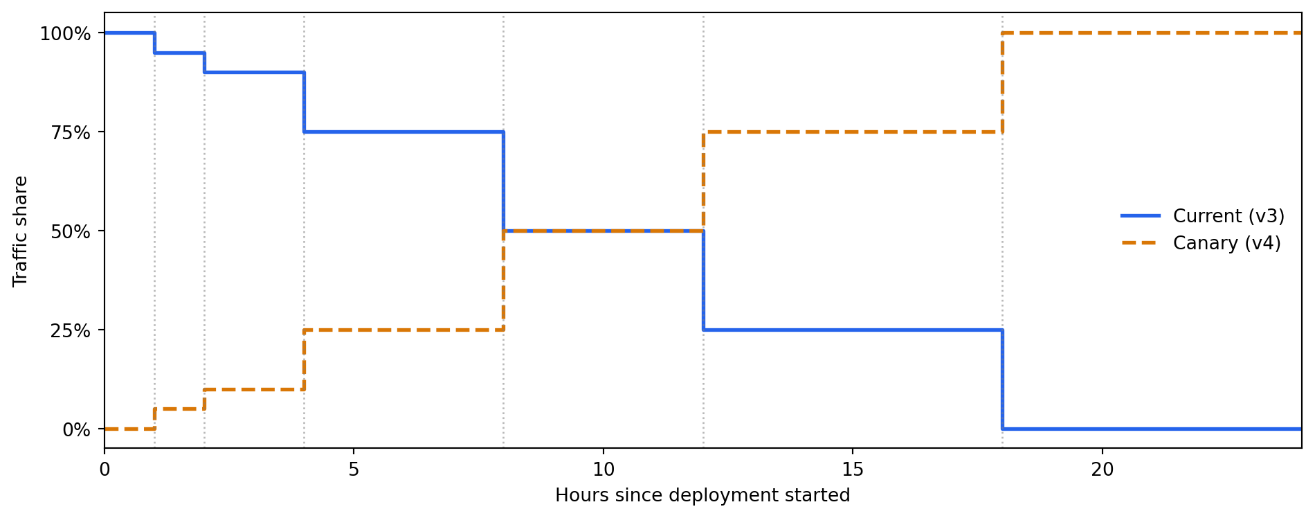
**Canary deployment** sends a small percentage of live traffic (say 5%) to the new model and the rest to the current one. You monitor both populations for differences in prediction distributions, downstream business metrics, and error rates. If the canary looks healthy, you gradually increase its traffic share. If anything looks wrong, you route all traffic back to the current model instantly. The rollback trigger should be defined *before* deployment starts: for example, "if the canary's mean predicted probability diverges by more than 2 standard errors of the mean (a measure of how precisely the mean is estimated) from the baseline over a 1-hour window, halt and roll back automatically." (The exact multiplier needs calibration for your traffic volume and acceptable false-alarm rate.)
**Blue/green deployment** maintains two complete serving environments. The "blue" environment runs the current model; the "green" environment runs the new one. A load balancer directs all traffic to blue. After validating green (via shadow or canary), you flip the load balancer to green. If problems emerge, flipping back to blue is a single configuration change.
All three strategies share a prerequisite: you must be able to **roll back quickly**. That means keeping the previous model artefact deployable, maintaining the prior serving environment, and testing the rollback procedure before you need it. A rollback you've never practised is a rollback that takes three hours at 2am.
```{python}
#| label: fig-canary-deployment
#| echo: true
#| fig-cap: "Simulated canary deployment. The new model (v4) starts at 0% of traffic
#| and rises to 5% after the first hour. As monitoring confirms healthy behaviour,
#| the traffic share increases over several hours until v4 handles all traffic."
#| fig-alt: "Step-line chart showing traffic share over a 24-hour canary rollout. The v3 (current) model starts at 100% and steps down through 95%, 90%, 75%, 50%, 25%, and 0% at hours 1, 2, 4, 8, 12, and 18 respectively. The v4 (canary) model starts at 0% and steps up through 5%, 10%, 25%, 50%, 75%, and 100% at the same decision points. Vertical dotted lines mark each traffic shift hour."
hours = np.array([0, 1, 2, 4, 8, 12, 18, 24])
v4_pct = np.array([0, 5, 10, 25, 50, 75, 100, 100])
v3_pct = 100 - v4_pct

fig, ax = plt.subplots(figsize=(10, 4))
fig.patch.set_alpha(0)
ax.patch.set_alpha(0)

ax.step(hours, v3_pct, where='post', label='Current (v3)', linewidth=2,
        color='#0072B2')
ax.step(hours, v4_pct, where='post', label='Canary (v4)', linewidth=2,
        linestyle='--', color='#E69F00')

# Mark decision points
for h in hours[1:-1]:
    ax.axvline(h, color='grey', linestyle=':', alpha=0.55, linewidth=1.0)

ax.set_xlabel('Hours since deployment started')
ax.set_ylabel('Traffic share (%)')
ax.set_yticks([0, 25, 50, 75, 100])
ax.set_yticklabels(['0%', '25%', '50%', '75%', '100%'])
ax.legend(frameon=False)
ax.set_xlim(0, 24)
ax.set_ylim(-5, 105)

# Strip spines for a cleaner look
for spine in ['top', 'right']:
    ax.spines[spine].set_visible(False)

plt.tight_layout()
plt.show()
```
::: {.callout-tip}
## Author's Note
The hardest thing about model deployment is that it breaks the most fundamental assumption of software deployment: that correctness is verifiable before you ship. In application code, tests are a pre-deployment oracle: if they pass, the system is correct by definition. With models, that relationship inverts. Every test can pass, every metric can look acceptable, and the deployed model can still make systematically worse decisions than its predecessor. There is no compiler error for "this model is subtly wrong about an important subpopulation."
Canary deployments are the engineering response to this inversion. They don't restore the pre-deployment oracle, but they transform deployment from a binary event into an observable process. The question shifts from "is this model correct?" (unanswerable before deployment) to "is this model behaving consistently with the current model on live data?" (answerable gradually). That's a weaker guarantee, but it's a real one.
:::
## Monitoring: the new failure modes {#sec-model-monitoring}
You already know how to watch for things going wrong: error spikes, latency, crashes. Model monitoring must also watch for things going *right but wrong*: the system is healthy by every infrastructure metric, but the predictions are degrading because the world has changed.
There are three layers of model monitoring, each catching a different class of problem.
**Infrastructure monitoring** is what you already know: CPU usage, memory, request latency, error rates, availability. If the model serving process is unhealthy, nothing else matters. Standard tools (Prometheus, Datadog, Grafana) handle this without modification.
**Data monitoring** watches the model's *inputs* for changes. If the distribution of incoming features shifts from what the model saw during training, predictions may become unreliable even though the model itself hasn't changed. This is **data drift** (also called **covariate shift** in the academic literature), a shift in $P(X)$, the same concept we validated against in @sec-data-validation, but now applied continuously to live traffic. Mechanically, drift detection is a *comparison of two distributions* — the training-time reference and the current production window — exactly the framing developed in @sec-distributions. The detection methods used in practice (KS tests, Population Stability Index, divergence measures) are operationalised hypothesis tests against the null that the two samples come from the same distribution.
**Performance monitoring** watches the model's *outputs* and, most importantly, its *outcomes*. Tracking predicted probability distributions catches some problems early; a sudden shift in mean prediction suggests something changed. But prediction distributions can shift due to data drift alone, without any decline in model quality. The definitive signal for **concept drift** — a change in the relationship between features and outcomes, $P(Y \mid X)$ (the probability of an outcome given the input features) — requires comparing predictions against ground-truth labels once they arrive. In many applications (fraud detection, churn prediction), labels arrive days or weeks after the prediction, making this a lagging but authoritative indicator.
```{python}
#| label: fig-data-drift
#| echo: true
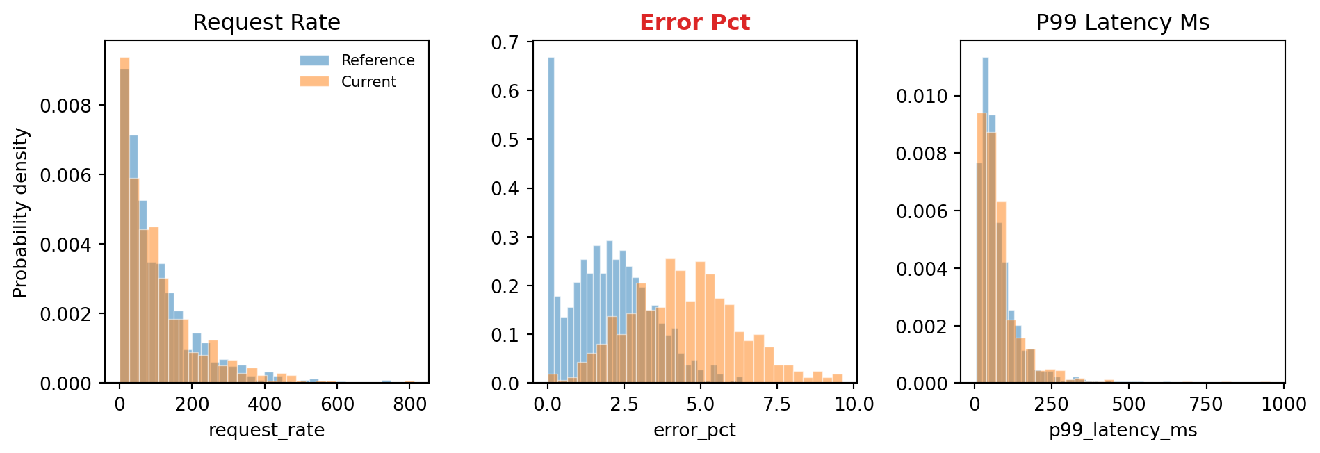
#| fig-cap: "Detecting data drift by comparing feature distributions between the
#| training data (reference) and recent production traffic (current). The
#| error_pct feature has drifted — its distribution has shifted right,
#| meaning incoming data now has higher error rates than the model was
#| trained on."
#| fig-alt: "Two overlapping histograms for each of three features arranged side by side. For request_rate and p99 Latency (ms), the reference (blue) and current (orange, hatched) histograms overlap substantially, indicating no drift. For error_pct, labelled 'Error Pct (drifted)' and visually emphasised, the current histogram is shifted visibly to the right of the reference, indicating drift. The p99 latency panel uses a log scale to accommodate the log-normal distribution."
rng_drift = np.random.default_rng(42)

# Simulate reference (training) distributions
ref_request_rate = rng_drift.exponential(100, 1000)
ref_error_pct = np.clip(rng_drift.normal(2, 1.5, 1000), 0, None)
ref_p99 = rng_drift.lognormal(4, 0.8, 1000)

# Simulate current (production) distributions — error_pct has drifted
cur_request_rate = rng_drift.exponential(105, 500)  # minor, within noise
cur_error_pct = np.clip(rng_drift.normal(4.5, 1.8, 500), 0, None)  # drifted!
cur_p99 = rng_drift.lognormal(4.1, 0.8, 500)  # minor shift

fig, axes = plt.subplots(1, 3, figsize=(10, 3.5))
fig.patch.set_alpha(0)

# Manual title map avoids .title() producing "P99 Latency Ms"
title_map = {
    'request_rate': 'Request Rate',
    'error_pct': 'Error Pct',
    'p99_latency_ms': 'p99 Latency (ms)',
}
drift_features = [
    ('request_rate', ref_request_rate, cur_request_rate),
    ('error_pct', ref_error_pct, cur_error_pct),
    ('p99_latency_ms', ref_p99, cur_p99),
]

for i, (ax, (name, ref, cur)) in enumerate(zip(axes, drift_features)):
    ax.patch.set_alpha(0)
    # Hatching differentiates series for colour-blind readers
    ax.hist(ref, bins=30, alpha=0.55, density=True, label='Reference',
            edgecolor='white', linewidth=0.5, color='#0072B2', hatch='')
    ax.hist(cur, bins=30, alpha=0.55, density=True, label='Current',
            edgecolor='white', linewidth=0.5, color='#E69F00', hatch='///')
    ax.set_xlabel(name)
    title = title_map[name]
    # Highlight the drifted panel with colour and "(drifted)" label
    if name == 'error_pct':
        ax.set_title(f"{title} (drifted)", color='#dc2626', fontweight='bold')
    else:
        ax.set_title(title)
    for spine in ['top', 'right']:
        ax.spines[spine].set_visible(False)

# p99_latency_ms is log-normal — log scale shows the distribution more clearly
axes[2].set_xscale('log')

axes[0].set_ylabel('Probability density')

# Single shared legend on the first panel only
axes[0].legend(fontsize=8, frameon=False)

plt.tight_layout()
plt.show()
```
As @fig-data-drift shows, the `error_pct` distribution in current traffic has shifted visibly to the right of the reference distribution. We can quantify this statistically. The **Kolmogorov–Smirnov (KS) test** compares two distributions and returns a test statistic (how different they are) and a p-value, measuring how often we would see a difference this large if both samples came from the same distribution. A low p-value signals meaningful drift:
```{python}
#| label: drift-detection
#| echo: true
from scipy import stats

# Reuse the reference and current distributions from the plot above
drift_pairs = {
    'request_rate': (ref_request_rate, cur_request_rate),
    'error_pct': (ref_error_pct, cur_error_pct),
    'p99_latency_ms': (ref_p99, cur_p99),
}

print(f"{'Feature':<20} {'KS statistic':>13} {'p-value':>12} {'Drift?':>8}")
print('-' * 57)
for name, (ref, cur) in drift_pairs.items():
    ks_stat, p_value = stats.ks_2samp(ref, cur)
    drifted = 'YES' if p_value < 0.01 else 'NO'
    p_str = f"{p_value:.2e}" if p_value < 0.001 else f"{p_value:.4f}"
    print(f"{name:<20} {ks_stat:>13.4f} {p_str:>12} {drifted:>8}")
```
The KS test flags `error_pct` as drifted: its distribution in current traffic is statistically different from the training distribution. The other two features show no significant shift. This doesn't necessarily mean the model is wrong, but it's a signal that warrants investigation. Perhaps an infrastructure change is causing more errors, or a new client is generating unusual traffic patterns.
One caveat about the KS test: it is designed for continuous distributions. Applied to discrete features such as `deploy_hour` or `is_weekend`, it is still informative but a chi-square test is more appropriate; use KS results for discrete features as a rough guide only.
A second caveat: when testing many features independently at the same significance threshold $\alpha$ (the per-test false-positive rate), the probability of at least one false alarm across $n$ tests is approximately $1 - (1 - \alpha)^n$ (this assumes the tests are independent; correlated features, which tend to drift together, make it a rough upper bound). With 20 features at $\alpha = 0.01$, that gives $1 - 0.99^{20} \approx 0.18$, roughly an 18% chance of a spurious drift flag even when nothing has changed. In practice, apply a Bonferroni correction (test each feature at $\alpha / n_\text{features}$ instead of $\alpha$) or track the KS statistic over time rather than hard-thresholding individual tests.
::: {.callout-note}
## Engineering Bridge
Data drift monitoring is the ML equivalent of **SLO-based alerting** in site reliability engineering. An SLO alert doesn't fire when a single request is slow — it fires when the error-budget consumption rate over a window is unsustainable, which amounts to monitoring a distributional statistic rather than individual events. Similarly, a drift alert doesn't fire when one input is unusual — it fires when the *distribution* of inputs has shifted enough that the model's assumptions may no longer hold.
:::
## CI/CD for machine learning {#sec-ml-cicd}
Software CI/CD pipelines test code: does it compile, do the unit tests pass, does the integration suite pass? ML CI/CD pipelines must also test *data and models*: is the data valid, does the model meet performance thresholds, do the predictions make sense?
A mature ML CI/CD pipeline has three layers of testing, each catching a different class of defect.
**Code tests** verify that the training and serving code works correctly, the same unit and integration tests you'd write for any software. Does the feature engineering function handle edge cases? Does the serving endpoint return the right schema? Does the pipeline run end-to-end on a small sample?
**Data tests** verify that the training data meets quality expectations, the validation checks from @sec-data-validation, now automated in CI. Are the required columns present? Are null rates within tolerance? Have distributions drifted beyond acceptable bounds?
**Model tests** verify that the trained model meets performance and behavioural expectations. These go beyond a single accuracy number:
```{python}
#| label: model-tests
#| echo: true
from sklearn.metrics import accuracy_score, f1_score

y_pred = pipeline.predict(X_test)
y_prob = pipeline.predict_proba(X_test)[:, 1]

# ---- Performance tests ----
accuracy = accuracy_score(y_test, y_pred)
f1 = f1_score(y_test, y_pred)

assert accuracy >= 0.65, f"Accuracy {accuracy:.4f} below threshold 0.65"
assert f1 >= 0.70, f"F1 {f1:.4f} below threshold 0.70"

# ---- Prediction distribution tests ----
# Predictions should not be degenerate (all same class)
unique_preds = np.unique(y_pred)
assert len(unique_preds) > 1, 'Model predicts only one class'

# Predicted probabilities should span a reasonable range
prob_range = y_prob.max() - y_prob.min()
assert prob_range > 0.3, f"Probability range {prob_range:.2f} too narrow"

print(f"All model tests passed:")
print(f"  Accuracy: {accuracy:.4f} (threshold: 0.65)")
print(f"  F1 score: {f1:.4f} (threshold: 0.70)")
print(f"  Probability range: {prob_range:.4f}")
```
A complete promotion suite would also include *directional tests* — assertions that moving a feature in the expected direction (e.g. higher error rate) moves the prediction in the expected direction. These catch a class of bugs that aggregate metrics miss: a model can hit 80% accuracy while getting the sign of an important feature backwards. We develop directional tests properly in @sec-directional-tests, alongside the other behavioural-test patterns (smoke, invariance, minimum-performance), and the same patterns plug straight into the promotion gate shown above.
::: {.callout-tip}
## Author's Note
Software engineering has a clean notion of correctness: a function satisfies its contract or it doesn't, and tests are the mechanism for checking this. Model correctness resists this framing. A model can satisfy every metric threshold (accuracy, precision, recall) and still violate fundamental domain logic, returning higher fraud scores for lower-risk inputs or recommending products to users who already own them. Aggregate metrics average over these failures and hide them.
Directional tests are a partial rescue: they encode domain knowledge as assertions and make violations visible. But they introduce a new responsibility that software engineers aren't used to: knowing enough about the domain to specify what "sensible" means. The test suite becomes a repository of domain knowledge, not just code contracts. That's a different relationship with tests than most engineers are used to.
:::
## The MLOps lifecycle {#sec-mlops-lifecycle}
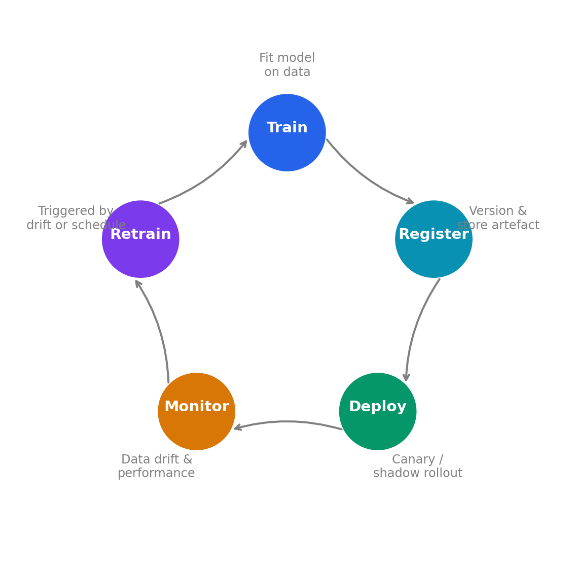
All of the components in this chapter connect into a continuous loop, shown in @fig-mlops-lifecycle. Training produces a model artefact, which is registered, deployed (via canary or shadow), monitored in production, and eventually retrained when drift is detected or new data arrives. This is the **MLOps lifecycle**, the ML equivalent of the CI/CD/monitoring feedback loop in DevOps. The loop runs clockwise: Train → Register → Deploy → Monitor → Retrain, with Retrain feeding back into Train.
```{python}
#| label: fig-mlops-lifecycle
#| echo: true
#| fig-cap: "The MLOps lifecycle. Training, registration, deployment, and monitoring
#| form a continuous loop. Drift detection or performance degradation triggers
#| retraining, closing the loop."
#| fig-alt: "A circular diagram with five stages arranged clockwise: Train (fit model on data), Register (version and store artefact), Deploy (canary or shadow rollout), Monitor (data drift, model performance), and Retrain (triggered by drift or schedule). Arrows connect each stage to the next in a continuous loop."
fig, ax = plt.subplots(figsize=(6, 6))
fig.patch.set_alpha(0)
ax.patch.set_alpha(0)

stages = ['Train', 'Register', 'Deploy', 'Monitor', 'Retrain']
descriptions = [
    'Fit model\non data',
    'Version &\nstore artefact',
    'Canary /\nshadow rollout',
    'Data drift &\nperformance',
    'Triggered by\ndrift or schedule',
]
# Accessible colour palette — Okabe-Ito, distinguishable under deuteranopia/protanopia
stage_colours = ['#0072B2', '#E69F00', '#009E73', '#D55E00', '#56B4E9']

n_stages = len(stages)
angles = np.linspace(np.pi/2, np.pi/2 - 2*np.pi, n_stages, endpoint=False)
radius = 2.5

for i, (stage, desc, angle) in enumerate(zip(stages, descriptions, angles)):
    x, y = radius * np.cos(angle), radius * np.sin(angle)

    circle = plt.Circle((x, y), 0.65, facecolor=stage_colours[i],
                         edgecolor='white', linewidth=2)
    ax.add_patch(circle)
    ax.text(x, y + 0.08, stage, ha='center', va='center',
            fontsize=11, fontweight='bold', color='white')

    # Description outside the circle — darkened to "0.3" for contrast
    desc_x = (radius + 1.1) * np.cos(angle)
    desc_y = (radius + 1.1) * np.sin(angle)
    ax.text(desc_x, desc_y, desc, ha='center', va='center',
            fontsize=9, color='0.3')

    # Arrow to next stage
    next_angle = angles[(i + 1) % n_stages]
    angle_start = angle - 0.25
    angle_end = next_angle + 0.25
    x1, y1 = radius * np.cos(angle_start), radius * np.sin(angle_start)
    x2, y2 = radius * np.cos(angle_end), radius * np.sin(angle_end)
    ax.annotate('', xy=(x2, y2), xytext=(x1, y1),
                arrowprops=dict(arrowstyle='->', color='0.3', lw=1.5,
                                connectionstyle='arc3,rad=0.15'))

ax.set_xlim(-4.5, 4.5)
ax.set_ylim(-4.5, 4.5)
ax.set_aspect('equal')
ax.axis('off')
fig.tight_layout()
plt.show()
```
The maturity of an MLOps practice can be gauged by how much of this loop is automated. At the lowest level, everything is manual: a data scientist trains in a notebook, copies the model file to a server, and checks Grafana dashboards when they remember. At the highest level, the entire loop is automated: a drift detector triggers retraining, CI validates the new model against performance thresholds and directional tests, the registry promotes the validated model, a canary deployment routes traffic, and monitoring closes the loop.
Most teams are somewhere in the middle, and that's fine. The right level of automation depends on how often the model changes, how critical it is, and how large the team is.
## A worked example: end-to-end deployment pipeline {#sec-mlops-worked-example}
The following example ties together the chapter's key components (validation gates, model registration, and drift detection) using the pipeline and test data from earlier in this chapter.
```{python}
#| label: deployment-pipeline
#| echo: true
import hashlib
import io
import joblib
from sklearn.metrics import accuracy_score, f1_score
from scipy import stats

# ---- 1. Validate (model tests) ----
y_pred = pipeline.predict(X_test)
y_prob = pipeline.predict_proba(X_test)[:, 1]
metrics = {
    'accuracy': round(accuracy_score(y_test, y_pred), 4),
    'f1': round(f1_score(y_test, y_pred), 4),
}
assert metrics['accuracy'] >= 0.65
assert metrics['f1'] >= 0.70
assert len(np.unique(y_pred)) > 1

# ---- 2. Register (hash the artefact) ----
buf = io.BytesIO()
joblib.dump(pipeline, buf)
model_hash = hashlib.sha256(buf.getvalue()).hexdigest()[:16]

registry_entry = {
    'model_name': 'incident-predictor',
    'version': 4,
    'model_hash': model_hash,
    'metrics': metrics,
    'status': 'staging',
    'training_samples': len(X_train),
}

# ---- 3. Pre-deployment drift check ----
# Compare training feature distributions against a recent production sample.
# The sample below is drawn from distributions close to training — small
# natural variation only, no meaningful drift — so the model can be promoted.
rng_prod = np.random.default_rng(99)
production_sample = np.column_stack([
    rng_prod.exponential(102, 300),
    np.clip(rng_prod.normal(2.1, 1.5, 300), 0, None),
    rng_prod.lognormal(4.02, 0.8, 300),
    rng_prod.integers(0, 24, 300),
    rng_prod.binomial(1, 2/7, 300),
])

feature_names = ['request_rate', 'error_pct', 'p99_latency_ms',
                 'deploy_hour', 'is_weekend']
drift_results = {}
for i, name in enumerate(feature_names):
    ks_stat, p_val = stats.ks_2samp(X_train[:, i], production_sample[:, i])
    drift_results[name] = {'ks_statistic': round(ks_stat, 4),
                           'p_value': round(p_val, 4),
                           'drifted': p_val < 0.01}

any_drift = any(d['drifted'] for d in drift_results.values())

# ---- 4. Promote (if all checks pass) ----
if not any_drift:
    registry_entry['status'] = 'production'

print('Deployment pipeline results:')
print(f"  Model: {registry_entry['model_name']} v{registry_entry['version']}")
print(f"  Accuracy: {metrics['accuracy']}, F1: {metrics['f1']}")
print(f"  Model hash: {model_hash}")
print(f"  Drift detected: {any_drift}")
print(f"  Status: {registry_entry['status']}")
print(f"\nDrift check details:")
for name, result in drift_results.items():
    flag = ' <- DRIFT' if result['drifted'] else ''
    print(f"  {name}: KS={result['ks_statistic']}, "
          f"p={result['p_value']}{flag}")
```
The pipeline follows the lifecycle: validate against performance thresholds, register with a content hash, check for drift against current production traffic, and promote to production only if all gates pass. In a real system, the promotion step would trigger a canary deployment rather than an immediate cutover.
## Summary {#sec-mlops-summary}
1. **Serialise the full pipeline, not just the model.** Packaging preprocessing and prediction into a single artefact eliminates train/serve skew and makes deployment a matter of swapping one file. Remember that the artefact carries no runtime environment — containerise the serving process to guarantee environment parity.
2. **Use a model registry.** Version your model artefacts the way you version container images — with metadata, lineage, and deployment status. This gives you auditability and fast rollback: reverting means re-promoting a previous version and redeploying.
3. **Choose the right deployment pattern.** Batch prediction covers most use cases and is simpler to operate. Real-time prediction adds latency constraints and scaling concerns. Canary and shadow deployments protect against the silent failure mode unique to models: wrong predictions that look correct.
4. **Monitor inputs, outputs, and outcomes.** Infrastructure monitoring catches serving failures. Data drift monitoring catches distribution shifts in the model's inputs. Performance monitoring — ultimately requiring ground-truth labels — catches degradation in the model's predictions. You need all three.
5. **Test models, not just code.** ML CI/CD adds data validation and model behavioural tests (performance thresholds, directional assertions) to the standard code testing pipeline. A model that passes all code tests can still produce harmful predictions.
## Exercises {#sec-mlops-exercises}
1. Write a function `validate_model(pipeline, X_test, y_test, thresholds)` that takes a fitted pipeline, test data, and a dictionary of metric thresholds (e.g., `{"accuracy": 0.70, "f1": 0.50}`), runs all specified metrics, and returns a dictionary with each metric's value and whether it passed. Add a directional test for at least one feature. Test it with a model that passes and one that fails (e.g., a `DummyClassifier`).
2. Implement a `detect_drift(reference, current, feature_names, alpha=0.01)` function that runs a KS test on each feature, returns a summary DataFrame with columns `[feature, ks_statistic, p_value, drifted]`, and prints a warning for any drifted features. Test it by generating a reference dataset and a current dataset where one feature has deliberately drifted.
3. Write a script that trains a model, serialises the full pipeline (scaler + model) using joblib, loads it back, and asserts that the loaded model produces identical predictions on a held-out test set. Measure the serialised file size and the load time. How would you reduce the artefact size for a model that needs to be deployed to a resource-constrained environment?
4. **Conceptual:** Your team deploys a fraud detection model via canary deployment, routing 5% of traffic to the new model. After 24 hours, the new model has flagged 30% more transactions as fraudulent than the old model. Is this a problem? What additional information would you need to decide whether to continue the rollout or roll back?
5. **Conceptual:** A colleague argues that model monitoring is unnecessary because "we retrain the model every week anyway, so drift doesn't matter." Under what conditions is weekly retraining sufficient? Under what conditions could a model degrade catastrophically between retraining cycles? What's the cheapest monitoring check you could add that would catch the most dangerous failures? Where does the DevOps CI/CD analogy break down when applied to ML — specifically, what can go wrong between deployments that has no equivalent in traditional software?