---
# Content: CC BY-NC-SA 4.0 | Code: MIT - see /LICENSE.md
title: "Fraud detection"
---
{{< include /_common-imports.qmd >}}
## The adversary in the data {#sec-fraud-intro}
You've defended systems against malicious actors before. SQL injection, cross-site scripting, privilege escalation: security engineering is fundamentally about anticipating how an intelligent adversary will exploit your system and building defences that hold up under deliberate attack. Fraud detection is the same problem applied to transactions rather than endpoints.
But there's a critical difference. In application security, you can often prevent the attack entirely: validate inputs, enforce authentication, patch the vulnerability. In fraud detection, you can't prevent fraudulent transactions from being *attempted*. The fraudster has already cleared your checkout flow, passed your authentication checks, and submitted a plausible-looking transaction. Your job is to distinguish the fraudulent ones from the legitimate ones — in real time, at scale, with extreme class imbalance, and against an adversary who adapts to every defence you deploy.
## The data: credit card transactions {#sec-fraud-data}
We'll simulate a dataset of credit card transactions with realistic properties: a low fraud rate, features derived from transaction metadata, and the kind of distributional differences between legitimate and fraudulent transactions that real fraud models exploit. The simulation captures the key statistical properties without requiring sensitive real-world data.
```{python}
#| label: fraud-data-setup
#| echo: true
#| code-fold: true
#| code-summary: "Expand to see transaction simulation code"
rng = np.random.default_rng(42)

n_legit = 9700
n_fraud = 300
n = n_legit + n_fraud

# Hour-of-day probability weights (unnormalised; divided by sum below)
# Legitimate: peaks during business hours, low overnight
legit_hour_weights = np.array([
    1, 1, 1, 1, 1, 2, 3, 5, 7, 8, 8, 7, 7, 6, 6, 5, 5, 5, 4, 4, 3, 3, 2, 1
], dtype=float)
legit_hour_probs = legit_hour_weights / legit_hour_weights.sum()

# Fraud: elevated overnight and late evening
fraud_hour_weights = np.array([
    6, 7, 7, 7, 6, 4, 3, 2, 2, 2, 2, 3, 3, 3, 3, 3, 4, 4, 4, 5, 5, 5, 5, 5
], dtype=float)
fraud_hour_probs = fraud_hour_weights / fraud_hour_weights.sum()

# Legitimate transactions
legit = pd.DataFrame({
    'amount_gbp': np.clip(rng.lognormal(3.2, 1.0, n_legit), 1, 5000).round(2),
    'hour_of_day': rng.choice(24, n_legit, p=legit_hour_probs),
    'distance_from_home_km': np.clip(rng.exponential(15, n_legit), 0, 500).round(1),
    'transactions_last_24h': rng.poisson(2.5, n_legit),
    'days_since_last_txn': np.clip(rng.exponential(1.5, n_legit), 0, 30).round(1),
    'is_online': rng.binomial(1, 0.45, n_legit),
    'is_foreign_currency': rng.binomial(1, 0.08, n_legit),
    'merchant_risk_score': np.clip(rng.beta(2, 8, n_legit), 0, 1).round(3),
    'is_fraud': 0,
})

# Fraudulent transactions — different distributional characteristics
fraud = pd.DataFrame({
    'amount_gbp': np.clip(rng.lognormal(4.5, 1.2, n_fraud), 5, 10000).round(2),
    'hour_of_day': rng.choice(24, n_fraud, p=fraud_hour_probs),
    'distance_from_home_km': np.clip(rng.exponential(80, n_fraud), 0, 2000).round(1),
    'transactions_last_24h': rng.poisson(6, n_fraud),
    'days_since_last_txn': np.clip(rng.exponential(0.4, n_fraud), 0, 10).round(1),
    'is_online': rng.binomial(1, 0.75, n_fraud),
    'is_foreign_currency': rng.binomial(1, 0.35, n_fraud),
    'merchant_risk_score': np.clip(rng.beta(5, 3, n_fraud), 0, 1).round(3),
    'is_fraud': 1,
})

txn = pd.concat([legit, fraud], ignore_index=True)
txn = txn.sample(frac=1, random_state=42).reset_index(drop=True)

# Engineered features
txn['is_night'] = ((txn['hour_of_day'] >= 23) | (txn['hour_of_day'] <= 4)).astype(int)
txn['amount_log'] = np.log1p(txn['amount_gbp'])
txn['txn_velocity_ratio'] = txn['transactions_last_24h'] / (txn['days_since_last_txn'] + 0.1)

print(f"Transactions: {n:,}")
print(f"Fraud rate: {txn['is_fraud'].mean():.1%}")
print(f"\nFeature summary (legitimate vs fraudulent):")
for col in ['amount_gbp', 'distance_from_home_km', 'transactions_last_24h', 'merchant_risk_score']:
    leg_mean = txn.loc[txn['is_fraud'] == 0, col].mean()
    fra_mean = txn.loc[txn['is_fraud'] == 1, col].mean()
    print(f"  {col:30s}  legit={leg_mean:8.1f}  fraud={fra_mean:8.1f}")
```
The 3% fraud rate is higher than typical production rates (which range from 0.1% to 1% depending on the industry), but low enough to exhibit the class imbalance challenges that dominate real fraud detection. The distributional differences we've embedded (higher amounts, more distant locations, higher transaction velocity, and more night-time activity for fraud) are the kind of statistical signals that real fraud models learn to exploit.
```{python}
#| label: fig-fraud-distributions
#| echo: true
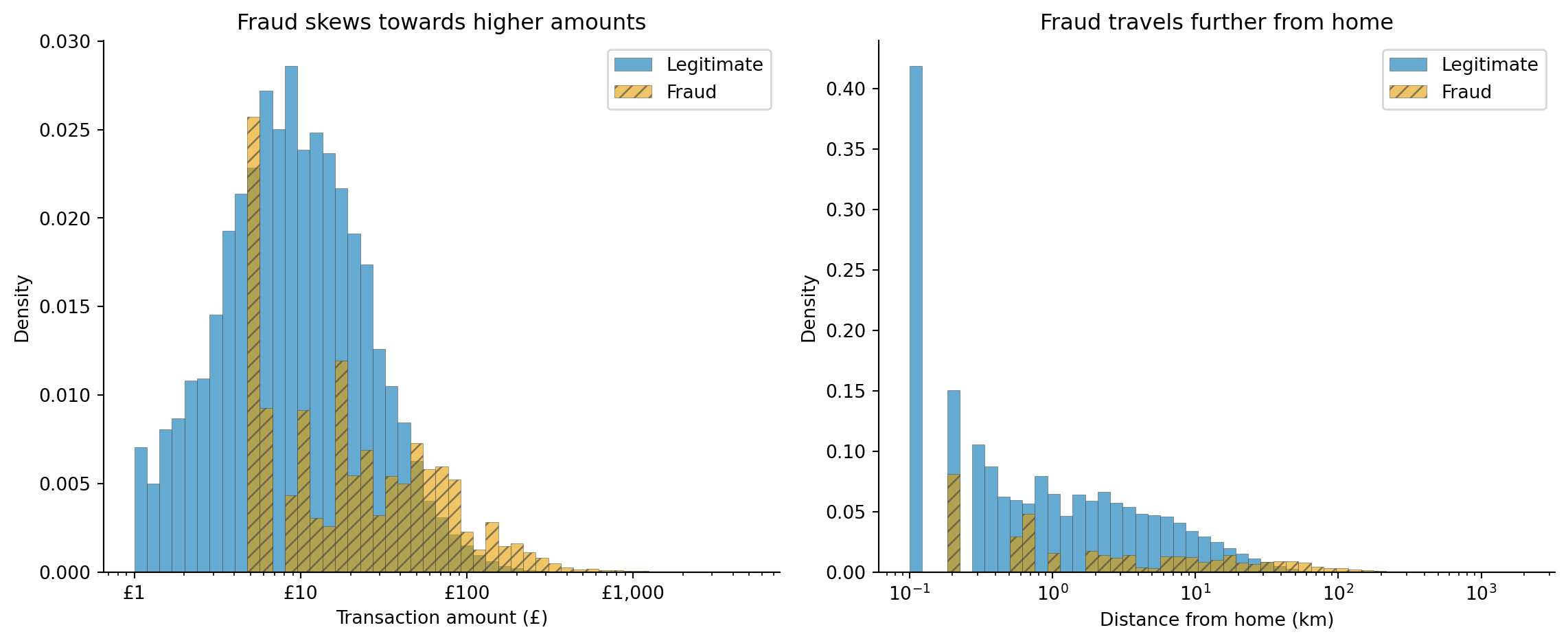
#| fig-cap: "Distribution of transaction amount and distance from home for legitimate and fraudulent transactions. Fraud transactions are systematically higher in both dimensions, but the distributions overlap substantially — there's no clean boundary."
#| fig-alt: "Two panels. Left: overlapping histograms of transaction amount in pounds on a log scale. The blue solid histogram for legitimate transactions peaks around 25 pounds while the orange hatched histogram for fraudulent transactions peaks around 90 pounds, but both distributions have wide tails that overlap extensively. Right: overlapping histograms of distance from home in kilometres on a log scale. Legitimate transactions cluster near zero with a steep exponential decay, while fraudulent transactions have a flatter distribution extending much further, on a log scale."
import matplotlib.ticker as mticker

fig, (ax1, ax2) = plt.subplots(1, 2, figsize=(12, 5))
fig.patch.set_alpha(0)

hatches = {0: '', 1: '///'}
for label, colour, name in [(0, '#0072B2', 'Legitimate'), (1, '#E69F00', 'Fraud')]:
    subset = txn[txn['is_fraud'] == label]
    ax1.hist(subset['amount_gbp'], bins=np.logspace(0, np.log10(5001), 50),
             alpha=0.6, color=colour, hatch=hatches[label],
             label=name, density=True, edgecolor='#444444', linewidth=0.3)
    ax2.hist(subset['distance_from_home_km'].clip(lower=0.1),
             bins=np.logspace(np.log10(0.1), np.log10(2001), 50),
             alpha=0.6, color=colour, hatch=hatches[label],
             label=name, density=True, edgecolor='#444444', linewidth=0.3)

ax1.set_xlabel('Transaction amount (£)')
ax1.set_ylabel('Density')
ax1.set_title('Fraud skews towards higher amounts')
ax1.set_xscale('log')
ax1.xaxis.set_major_formatter(mticker.FuncFormatter(lambda x, _: f'£{x:,.0f}'))
ax1.legend(loc='upper right')
ax1.spines[['top', 'right']].set_visible(False)
ax1.patch.set_alpha(0)

ax2.set_xlabel('Distance from home (km)')
ax2.set_ylabel('Density')
ax2.set_title('Fraud travels further from home')
ax2.set_xscale('log')
ax2.legend(loc='upper right')
ax2.spines[['top', 'right']].set_visible(False)
ax2.patch.set_alpha(0)

plt.tight_layout()
plt.show()
```
The overlap in @fig-fraud-distributions is the core challenge. If fraudulent transactions always had amounts above £500 or distances above 200 km, a simple rule engine would suffice. The distributions overlap because fraudsters deliberately make transactions look normal: many fraudulent transactions are moderate amounts at plausible-looking merchants. A model must learn the *joint* distribution of multiple features, not just threshold individual ones.
::: {.callout-note}
## Engineering Bridge
Fraud detection and intrusion detection share the same fundamental structure: classify events as benign or malicious in a high-throughput stream where the vast majority are benign. The features differ (transaction amounts versus packet headers) but the challenges are identical: extreme class imbalance, asymmetric costs (false negatives are far worse than false positives), and an adversary who studies your defences and adapts. If you've written firewall rules or tuned an intrusion detection system (IDS), you've already dealt with the tension between catching threats and flooding the security team with false positives. The analogy breaks down at the cost of a false positive: a dropped packet gets retried transparently, but a declined payment interrupts a customer mid-purchase, a visible, friction-generating event with direct revenue consequences.
:::
## The class imbalance problem {#sec-fraud-imbalance}
At 3% fraud, a model that predicts "legitimate" for every transaction achieves 97% accuracy. This is the accuracy paradox from @sec-class-imbalance: high accuracy, zero usefulness. The model catches no fraud at all, which is precisely the worst possible outcome.
Class imbalance affects every stage of the pipeline. During training, with roughly 32 legitimate examples for every fraudulent one, the loss function is dominated by the majority class: the model optimises for getting legitimate transactions right because that's where most of the error signal comes from. During evaluation, accuracy is misleading because it's dominated by the majority class. During deployment, the base rate produces a surprising arithmetic: even a model with 90% precision still flags one legitimate transaction for every nine genuine fraud catches — and once precision falls below 50%, which is common at a 3% base rate, the absolute number of false positives outnumbers the number of true positives. This base rate effect is a direct consequence of Bayes' theorem, as discussed in @sec-precision-recall-tradeoff, and it routinely trips up engineering teams who focus on precision in isolation.
We'll compare two approaches to handling imbalance: training on the raw data (letting the algorithm deal with skew) and adjusting class weights (penalising errors on the minority class more heavily). A third common approach (SMOTE, which synthesises new minority-class examples) exists but adds a dependency and doesn't always outperform well-tuned class weights. We'll focus instead on threshold tuning as the primary lever for controlling the fraud-vs-friction trade-off after training.
```{python}
#| label: fraud-train-test-split
#| echo: true
from sklearn.model_selection import train_test_split

feature_cols = ['amount_log', 'hour_of_day', 'distance_from_home_km',
                'transactions_last_24h', 'days_since_last_txn', 'is_online',
                'is_foreign_currency', 'merchant_risk_score', 'is_night',
                'txn_velocity_ratio']

X = txn[feature_cols]
y = txn['is_fraud']

# Stratified split to preserve class ratio in both sets
X_train, X_test, y_train, y_test = train_test_split(
    X, y, test_size=0.3, random_state=42, stratify=y
)

print(f"Training set: {len(X_train):,} transactions ({y_train.mean():.1%} fraud)")
print(f"Test set:     {len(X_test):,} transactions ({y_test.mean():.1%} fraud)")
```
We'll evaluate both strategies using **average precision** (AP), a metric that summarises the precision-recall curve and is far more informative than accuracy for imbalanced problems. We'll unpack AP in detail after the comparison.
```{python}
#| label: fraud-imbalance-strategies
#| echo: true
from sklearn.ensemble import GradientBoostingClassifier
from sklearn.metrics import classification_report, average_precision_score

# Strategy 1: No adjustment — raw imbalanced data
gbm_raw = GradientBoostingClassifier(
    n_estimators=200, learning_rate=0.1, max_depth=4, random_state=42
)
gbm_raw.fit(X_train, y_train)

# Strategy 2: Class weights — penalise minority-class errors
# GradientBoostingClassifier doesn't have class_weight, so we use sample_weight.
# (The newer HistGradientBoostingClassifier supports class_weight='balanced' directly.)
# Weight fraud examples by the inverse class frequency in the training set.
neg_count = (y_train == 0).sum()
pos_count = (y_train == 1).sum()
weights = np.where(y_train == 1, neg_count / pos_count, 1.0)
gbm_weighted = GradientBoostingClassifier(
    n_estimators=200, learning_rate=0.1, max_depth=4, random_state=42
)
gbm_weighted.fit(X_train, y_train, sample_weight=weights)

# Compare on test set
for name, model in [('Raw (no adjustment)', gbm_raw),
                     ('Class-weighted', gbm_weighted)]:
    y_prob = model.predict_proba(X_test)[:, 1]
    ap = average_precision_score(y_test, y_prob)
    print(f"\n{name}:")
    print(f"  Average precision (AP): {ap:.3f}")
    print(classification_report(y_test, model.predict(X_test),
                                target_names=['Legitimate', 'Fraud'],
                                digits=3, zero_division=0))
```
How does AP work? It computes the weighted mean of precision values at each threshold, where the weight is the *increase* in recall achieved by lowering the threshold to that point, approximating the area under the precision-recall curve. A model that achieves high precision only at very low recall (catching a few fraudsters with perfect accuracy but missing most) scores poorly on AP, which is exactly the behaviour you want to penalise. Unlike the ROC curve's AUC (@sec-roc-auc), which plots recall against the false positive rate (FPR = FP / (FP + TN)) on its x-axis, AP uses precision, which excludes true negatives entirely. When the negative class is enormous, FPR is diluted: even a large number of false positives produces a small FPR because TN dwarfs them, making AUC look optimistic; AP does not suffer from this inflation. For imbalanced problems, AP is the metric to watch.
::: {.callout-tip}
## Author's Note
The surprising thing about class imbalance wasn't any individual technique but realising that class weights, oversampling, and threshold adjustment are three framings of the same underlying problem, not three separate solutions. My engineering instinct was to pick the right tool for the job and move on. But in fraud detection, these approaches operate at different stages of the pipeline (training, data preparation, and decision time) and they interact. The conceptual shift was accepting that the model and the decision rule are separate concerns. The model learns to score; the threshold decides what to do about it. Separating them gives you operational control you don't get if you bake the trade-off into the training process.
:::
## Choosing the right threshold {#sec-fraud-threshold}
A fraud model doesn't output "fraud" or "not fraud"; it outputs a probability. The threshold that converts probability to decision is separate from the model, and it encodes a business trade-off: how many legitimate customers are you willing to inconvenience (false positives) to catch each additional fraudster (true positives)?
This is the same precision-recall trade-off from @sec-precision-recall-tradeoff, but the stakes are sharper. Every false positive is a legitimate customer whose card is declined or whose transaction is delayed for manual review, a direct hit to customer experience. Every false negative is a fraudulent transaction that goes through, a direct financial loss.
```{python}
#| label: fig-fraud-precision-recall
#| echo: true
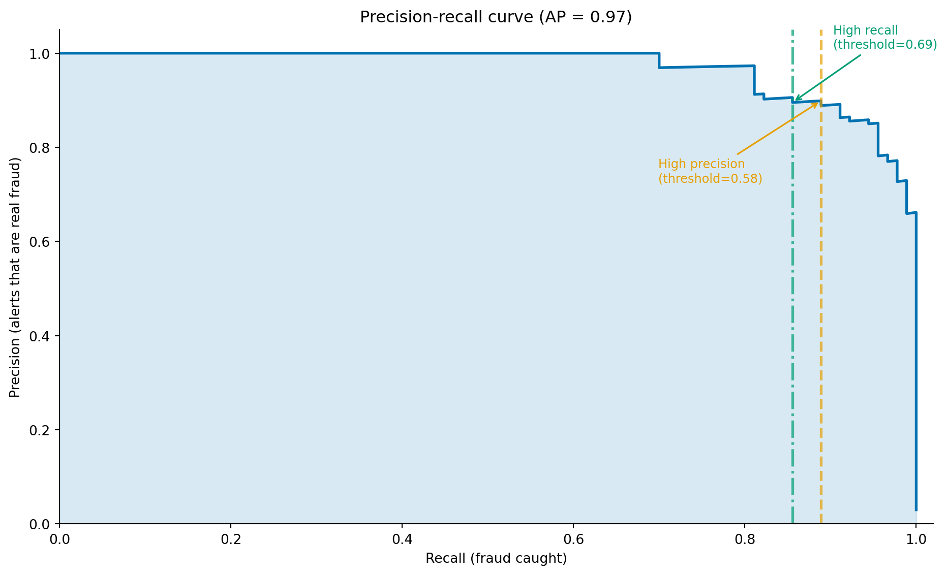
#| fig-cap: "Precision-recall curve for the class-weighted gradient boosting model. The dashed lines mark two operating points: a high-precision threshold that blocks few legitimate transactions but misses some fraud, and a high-recall threshold that catches more fraud at the cost of more false positives."
#| fig-alt: "Precision-recall curve showing precision on the vertical axis and recall on the horizontal axis. The curve starts near precision 1.0 at low recall and drops as recall increases. A dashed orange vertical line marks the high-precision operating point at recall around 0.6 with a threshold annotation, and a dash-dot green vertical line marks the high-recall operating point at recall around 0.85 with a threshold annotation. Arrows connect each line to an annotation showing the threshold value. The area under the curve is shaded in light blue."
from sklearn.metrics import precision_recall_curve

y_scores = gbm_weighted.predict_proba(X_test)[:, 1]
precision, recall, thresholds = precision_recall_curve(y_test, y_scores)

fig, ax = plt.subplots(figsize=(10, 6))
fig.patch.set_alpha(0)
ax.patch.set_alpha(0)
ax.fill_between(recall, precision, alpha=0.15, color='#0072B2')
ax.plot(recall, precision, color='#0072B2', linewidth=2)

# Mark two operating points
# precision/recall arrays have one extra element; [:-1] aligns with thresholds
high_prec_idx = np.argmin(np.abs(precision[:-1] - 0.90))
high_rec_idx = np.argmin(np.abs(recall[:-1] - 0.85))

ax.axvline(recall[high_prec_idx], color='#E69F00', linestyle='--', linewidth=2, alpha=0.7)
ax.annotate(f'High precision\n(threshold={thresholds[high_prec_idx]:.2f})',
            xy=(recall[high_prec_idx], precision[high_prec_idx]),
            xytext=(-120, -60), textcoords='offset points', fontsize=9, color='#E69F00',
            arrowprops=dict(arrowstyle='->', color='#E69F00', lw=1.2))

ax.axvline(recall[high_rec_idx], color='#009E73', linestyle='-.', linewidth=2, alpha=0.7)
ax.annotate(f'High recall\n(threshold={thresholds[high_rec_idx]:.2f})',
            xy=(recall[high_rec_idx], precision[high_rec_idx]),
            xytext=(30, 40), textcoords='offset points', fontsize=9, color='#009E73',
            arrowprops=dict(arrowstyle='->', color='#009E73', lw=1.2))

ap = average_precision_score(y_test, y_scores)
ax.set_xlabel('Recall (fraud caught)')
ax.set_ylabel('Precision (alerts that are real fraud)')
ax.set_title(f'Precision-recall curve (AP = {ap:.2f})')
ax.set_xlim(0, 1.02)
ax.set_ylim(0, 1.05)
ax.spines[['top', 'right']].set_visible(False)
plt.tight_layout()
plt.show()
```
The two operating points in @fig-fraud-precision-recall represent genuinely different business strategies. The high-precision point blocks fewer legitimate transactions but lets more fraud through, suitable for a low-friction payment flow where customer experience is paramount. The high-recall point catches more fraud but generates more false positives, suitable for high-value transactions or regulatory environments where fraud losses carry severe penalties.
One important subtlety: the cost calculation assumes the model's predicted probabilities are well-calibrated: that a transaction scored at 0.4 actually has about a 40% chance of being fraudulent. Gradient boosting models are often poorly calibrated out of the box; if calibration matters (and in cost-sensitive decisions it does), apply Platt scaling or isotonic regression to the raw scores before using them for threshold selection.
In production, this isn't a single threshold. Most fraud systems use tiered decisions: transactions scoring below 0.2 are approved automatically, those between 0.2 and 0.6 trigger automated friction (address verification, a 3D Secure challenge) before approval, and those above 0.6 are held for manual review. The thresholds at each tier are different business decisions with different cost structures.
## The economics of fraud detection {#sec-fraud-economics}
The right threshold depends on the relative costs of each outcome. Suppose each false negative (missed fraud) costs £150 on average (the transaction amount plus investigation costs plus chargeback fees), and each false positive costs £5 (the revenue lost from a declined legitimate transaction plus the customer goodwill damage). At the default 0.5 threshold, a typical fraud model might catch, say, 70% of fraud while declining a couple of percent of legitimate transactions. Is that the right trade-off?
We can compute the expected cost at each threshold, just as we did for the inventory quantile in @sec-demand-costs. Let $c_{\text{FN}}$ be the cost per missed fraud (false negative) and $c_{\text{FP}}$ the cost per incorrectly declined legitimate transaction (false positive). At any threshold, the model produces $\text{FN}$ false negatives and $\text{FP}$ false positives, giving a total cost of:
$$
\text{Total cost} = c_{\text{FN}} \times \text{FN} + c_{\text{FP}} \times \text{FP}
$$
In other words: sum the cost of every missed fraud plus the cost of every wrongly declined legitimate transaction at that threshold. Slide the threshold and the mix of FN and FP changes; the optimal threshold is wherever this sum is smallest.
The absolute cost depends on the size of the evaluation set: what transfers to production is the *threshold location*, not the pound figure. The cost numbers below are computed on our 3,000-transaction test set; the optimal threshold would be the same on a larger dataset with the same fraud rate.
```{python}
#| label: fig-fraud-cost-curve
#| echo: true
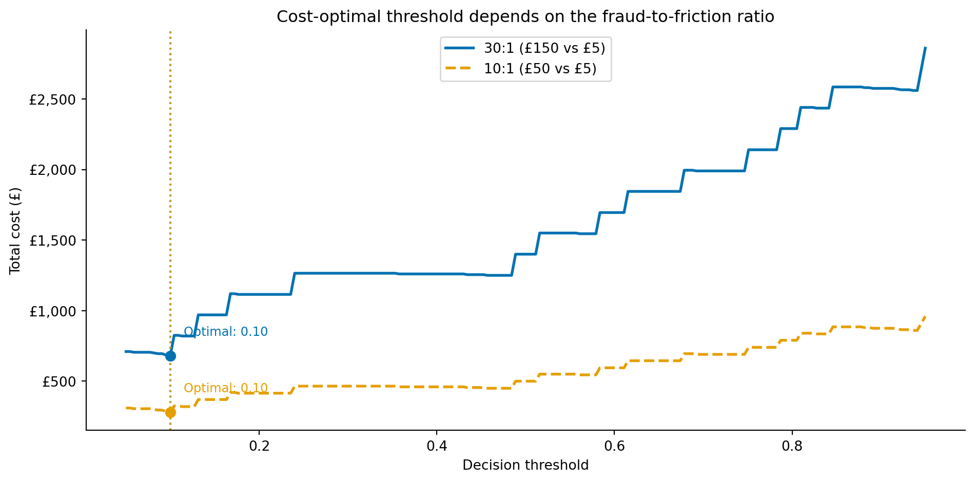
#| fig-cap: "Total cost on the test set as a function of the decision threshold for two cost scenarios. The cost-minimising threshold shifts depending on the relative cost of missed fraud versus false alarms. These costs are computed from the model's uncalibrated, class-weighted scores, so the threshold shown is illustrative; calibrate the probabilities (for example with `CalibratedClassifierCV`) before acting on a specific cut-off."
#| fig-alt: "Line chart with two cost curves. The horizontal axis is the decision threshold from 0 to 1. The vertical axis is total cost in pounds. The solid blue curve for the 30:1 cost ratio (150 pounds missed fraud versus 5 pounds false positive) is lowest at the aggressive low-threshold end of the range, then rises as the threshold increases and more fraud is missed. The dashed orange curve for the 10:1 cost ratio follows a similar shape with a shallower trough, also minimised at the aggressive low-threshold end. Vertical dotted lines mark the optimal threshold for each scenario, both at the aggressive low-threshold end of the range."
thresholds_range = np.linspace(0.05, 0.95, 200)

fig, ax = plt.subplots(figsize=(10, 5))
fig.patch.set_alpha(0)
ax.patch.set_alpha(0)

for c_fn, c_fp, label, colour, ls in [
    (150, 5, '30:1 (£150 vs £5)', '#0072B2', '-'),
    (50, 5, '10:1 (£50 vs £5)',  '#E69F00', '--'),
]:
    costs = []
    for t in thresholds_range:
        y_pred_t = (y_scores >= t).astype(int)
        fn = ((y_test == 1) & (y_pred_t == 0)).sum()
        fp = ((y_test == 0) & (y_pred_t == 1)).sum()
        costs.append(c_fn * fn + c_fp * fp)

    costs = np.array(costs)
    best_t = thresholds_range[np.argmin(costs)]
    ax.plot(thresholds_range, costs, linewidth=2, label=f'{label}', color=colour,
            linestyle=ls)
    ax.axvline(best_t, color=colour, linestyle=':', alpha=0.8, linewidth=1.5)
    ax.plot(best_t, costs.min(), 'o', color=colour, zorder=5, markersize=7)
    ax.annotate(f'Optimal: {best_t:.2f}', xy=(best_t, costs.min()),
                xytext=(10, 15), textcoords='offset points', fontsize=9,
                color=colour)

ax.set_xlabel('Decision threshold')
ax.set_ylabel('Total cost (£)')
ax.yaxis.set_major_formatter(mticker.FuncFormatter(lambda x, _: f'£{x:,.0f}'))
ax.set_title('Cost-optimal threshold depends on the fraud-to-friction ratio')
ax.legend(loc='upper center')
ax.spines[['top', 'right']].set_visible(False)
plt.tight_layout()
plt.show()
```
When missed fraud is expensive relative to false alarms (the 30:1 scenario), the optimal threshold is low: flag aggressively, accept more false positives. As the ratio shrinks (10:1), the penalty for raising the threshold eases — the cost curve's trough becomes shallower, so a higher cut-off costs little extra even when the minimum stays at the aggressive end, as it does here for this well-separated model. This is the same economic logic as the newsvendor model in @sec-demand-costs, applied to a classification boundary rather than an inventory quantile.
::: {.callout-note}
## Engineering Bridge
Threshold economics in fraud detection mirrors **alert tuning** in operations. A noisy alerting system generates alert fatigue: on-call engineers start ignoring pages, and real incidents get lost in the noise. A quiet alerting system misses genuine failures. The art of alert tuning is setting thresholds that balance sensitivity (catching real incidents) against specificity (not waking someone at 3 a.m. for a false positive). Fraud detection is the same problem with financial costs attached: too many false positives and you lose customers; too few and you lose money. The solution in both domains is to quantify the costs on each side and set the threshold where total expected cost is minimised, then monitor continuously because the cost landscape shifts as fraud patterns and business conditions change.
:::
## Feature importance and model interpretability {#sec-fraud-interpretability}
Catching fraud isn't enough; you need to explain *why* a transaction was flagged. Regulatory requirements (such as GDPR Article 22, which grants individuals the right to contest automated decisions, and similar frameworks in other jurisdictions) may require that customers be told why a transaction was declined. Internal fraud analysts reviewing flagged transactions need to understand the model's reasoning to investigate efficiently. And model developers need to verify that the model is learning genuine fraud signals rather than artefacts of the training data.
```{python}
#| label: fig-fraud-importance
#| echo: true
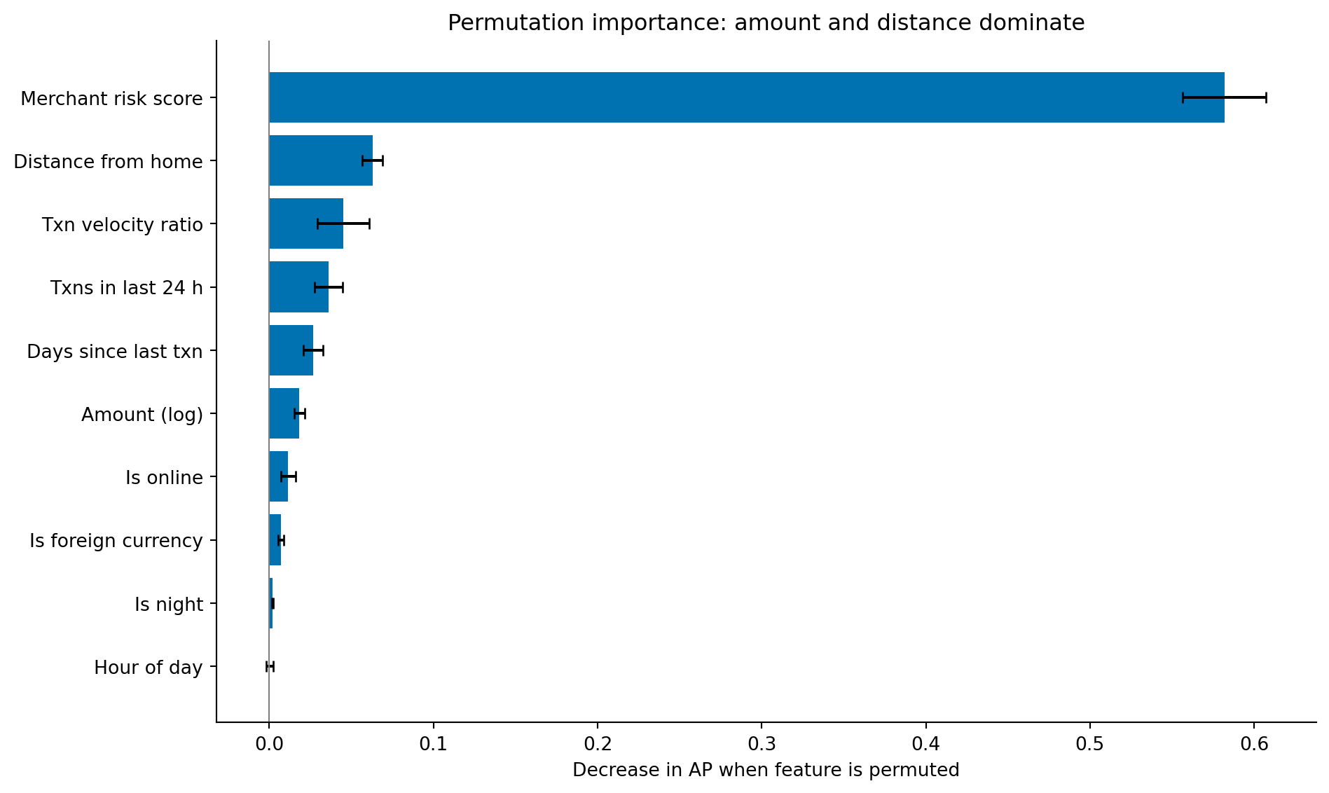
#| fig-cap: "Permutation importance for the fraud detection model. The merchant risk score dominates by a wide margin; distance from home and the transaction-velocity features follow well behind, while transaction amount ranks only mid-table."
#| fig-alt: "Horizontal bar chart showing permutation importance for ten features in the fraud detection model. One bar dominates: merchant risk score, roughly nine times longer than the next. From there the bars drop sharply and shorten gradually: distance from home, transaction velocity ratio, transactions in last 24 hours, days since last transaction, amount (log), is online, is foreign currency, is night, and hour of day. Error bars show standard deviation across permutation repeats."
from sklearn.inspection import permutation_importance

perm = permutation_importance(gbm_weighted, X_test, y_test, n_repeats=10,
                              random_state=42, scoring='average_precision')

sorted_idx = np.argsort(perm.importances_mean)

# Human-readable labels for the chart
display_names = {
    'amount_log': 'Amount (log)',
    'hour_of_day': 'Hour of day',
    'distance_from_home_km': 'Distance from home',
    'transactions_last_24h': 'Txns in last 24 h',
    'days_since_last_txn': 'Days since last txn',
    'is_online': 'Is online',
    'is_foreign_currency': 'Is foreign currency',
    'merchant_risk_score': 'Merchant risk score',
    'is_night': 'Is night',
    'txn_velocity_ratio': 'Txn velocity ratio',
}
labels = [display_names.get(feature_cols[i], feature_cols[i]) for i in sorted_idx]

fig, ax = plt.subplots(figsize=(10, 6))
fig.patch.set_alpha(0)
ax.patch.set_alpha(0)
ax.barh(range(len(sorted_idx)), perm.importances_mean[sorted_idx],
        xerr=perm.importances_std[sorted_idx],
        color='#0072B2', edgecolor='none', capsize=3)
ax.axvline(0, color='grey', linewidth=0.8, linestyle='-')  # zero reference
ax.set_yticks(range(len(sorted_idx)))
ax.set_yticklabels(labels)
ax.set_xlabel('Decrease in AP when feature is permuted')
ax.set_title('Permutation importance: merchant risk score dominates')
ax.spines[['top', 'right']].set_visible(False)
plt.tight_layout()
plt.show()
```
The ranking is led, decisively, by the merchant risk score: permuting it degrades the model roughly nine times as much as permuting the next feature. That fits the data — fraudulent transactions concentrate at higher-risk merchants — and it fits how the score is built, as a single clean signal that no other feature duplicates. Distance from home and the velocity features (the transaction-velocity ratio and the raw 24-hour count, which together capture the common fraud pattern of rapid successive charges) follow well behind. Transaction amount, which domain intuition might place near the top, lands only mid-table: fraudulent and legitimate amounts overlap heavily (@fig-fraud-distributions), so amount carries less standalone discriminative power than its prominence in fraud folklore suggests.
The velocity ratio and the raw 24-hour count illustrate the same correlated-feature caveat we met with the demand model (@sec-demand-drivers): because they encode overlapping information, permutation importance under-credits each of them individually. Read them as a group rather than ranking one against the other.
This interpretability check also serves as a sanity test. If the most important feature were `hour_of_day`, far exceeding merchant risk score or distance, you'd want to investigate whether the model was exploiting a data artefact rather than a genuine fraud signal. Feature importance that contradicts domain knowledge is a warning sign, not a discovery; it usually means the model has found a shortcut in the training data rather than a genuine fraud signal.
## Adversarial drift: when the rules change {#sec-fraud-drift}
Here's where fraud detection diverges from most classification problems. Churn (see @sec-churn-pipeline) is a *near-stationary* problem: customer behaviour evolves over months, but it does not evolve in response to your model's predictions. Fraud is the opposite — the data-generating process changes *because of your model*. Both pipelines share the same machinery (class imbalance, threshold selection, cost-aware decisions), but the monitoring and retraining cadence differ sharply: where churn can usually tolerate monthly retrains, fraud often cannot. Fraudsters adapt. When the model learns to flag high-amount overnight transactions, fraudsters switch to smaller daytime transactions. When it flags foreign-currency purchases, they use domestic cards. The relationship between features and the target is **non-stationary**, and the non-stationarity is adversarial: it specifically targets whatever signal your current model relies on.
This means a fraud model's performance degrades not just through ordinary distribution drift (which @sec-model-monitoring covers) but through deliberate evasion. We can simulate this to see how a model trained on one fraud pattern performs when the pattern changes.
```{python}
#| label: fraud-drift-simulation
#| echo: true
from sklearn.metrics import recall_score

# Separate RNG for drift scenario — keeps results independent of earlier draws
rng_drift = np.random.default_rng(99)

# Simulate a drift scenario: fraudsters shift to lower amounts and closer distances
# after learning that the model flags high-amount, distant transactions
fraud_shifted = pd.DataFrame({
    'amount_gbp': np.clip(rng_drift.lognormal(3.5, 0.8, 200), 5, 2000).round(2),
    'hour_of_day': rng_drift.choice(24, 200),  # uniform — shifted from night-time pattern
    'distance_from_home_km': np.clip(rng_drift.exponential(25, 200), 0, 300).round(1),
    'transactions_last_24h': rng_drift.poisson(4, 200),
    'days_since_last_txn': np.clip(rng_drift.exponential(0.8, 200), 0, 10).round(1),
    'is_online': rng_drift.binomial(1, 0.80, 200),
    'is_foreign_currency': rng_drift.binomial(1, 0.10, 200),
    'merchant_risk_score': np.clip(rng_drift.beta(3, 4, 200), 0, 1).round(3),
    'is_fraud': 1,
})

# Add the same engineered features
fraud_shifted['is_night'] = ((fraud_shifted['hour_of_day'] >= 23) |
                              (fraud_shifted['hour_of_day'] <= 4)).astype(int)
fraud_shifted['amount_log'] = np.log1p(fraud_shifted['amount_gbp'])
fraud_shifted['txn_velocity_ratio'] = (fraud_shifted['transactions_last_24h'] /
                                        (fraud_shifted['days_since_last_txn'] + 0.1))

# Sample fresh legitimate transactions from the full dataset (not just test set)
legit_new = txn[txn['is_fraud'] == 0].sample(2000, random_state=99)
drift_data = pd.concat([legit_new, fraud_shifted], ignore_index=True)

# Score with the original model
drift_scores = gbm_weighted.predict_proba(drift_data[feature_cols])[:, 1]
drift_preds = (drift_scores >= 0.5).astype(int)
drift_actual = drift_data['is_fraud']

# Compare performance
original_recall = recall_score(y_test, (y_scores >= 0.5).astype(int))
drift_recall = recall_score(drift_actual, drift_preds)

print(f"Recall on original test data:  {original_recall:.3f}")
print(f"Recall after adversarial drift: {drift_recall:.3f}")
print(f"Drop in recall: {original_recall - drift_recall:+.3f}")
```
The recall drop quantifies what happens when the model encounters fraud patterns it hasn't seen. This isn't a hypothetical; it's the fundamental operational challenge of fraud detection. The model's performance at deployment is a *ceiling*; adversarial adaptation ensures it degrades from there.
```{python}
#| label: fig-fraud-drift-comparison
#| echo: true
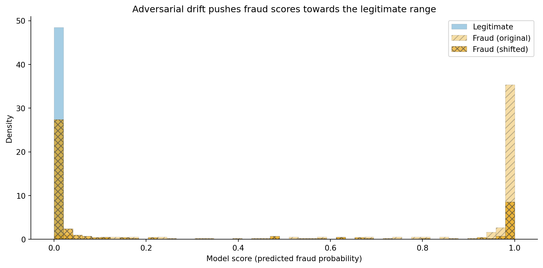
#| fig-cap: "Score distributions for original and shifted fraud patterns. After adversarial drift, fraudulent transactions score lower — closer to the legitimate distribution — making them harder for the model to catch at any threshold."
#| fig-alt: "Three overlapping histograms showing the model's predicted fraud probability. The blue solid histogram for legitimate transactions (2,910 samples) is concentrated near zero. The orange hatched histogram for original fraud patterns (90 samples) is concentrated near one. The vermillion cross-hatched histogram for shifted fraud patterns (200 samples) is spread broadly between 0.2 and 0.8, overlapping heavily with both other distributions — showing that the model struggles to distinguish the new fraud pattern."
fig, ax = plt.subplots(figsize=(10, 5))
fig.patch.set_alpha(0)
ax.patch.set_alpha(0)

bins = np.linspace(0, 1, 50)
ax.hist(y_scores[y_test == 0], bins=bins, alpha=0.35, color='#0072B2',
        hatch='', label='Legitimate', density=True, edgecolor='#444444', linewidth=0.3)
ax.hist(y_scores[y_test == 1], bins=bins, alpha=0.35, color='#E69F00',
        hatch='///', label='Fraud (original)', density=True, edgecolor='#444444', linewidth=0.3)

shifted_scores = gbm_weighted.predict_proba(fraud_shifted[feature_cols])[:, 1]
ax.hist(shifted_scores, bins=bins, alpha=0.65, color='#D55E00',
        hatch='xxx', label='Fraud (shifted)', density=True, edgecolor='#444444', linewidth=0.3)

ax.set_xlabel('Model score (predicted fraud probability)')
ax.set_ylabel('Density')
ax.set_title('Adversarial drift pushes fraud scores towards the legitimate range')
ax.legend()
ax.spines[['top', 'right']].set_visible(False)
plt.tight_layout()
plt.show()
```
The score distribution in @fig-fraud-drift-comparison makes the problem visual. The original fraud pattern (orange, hatched) separates cleanly from legitimate transactions (blue, solid). The shifted pattern (vermillion, cross-hatched) overlaps heavily: the fraudsters have moved into the region of feature space where the model can't distinguish them. No threshold adjustment can fix this; the model needs to be retrained on examples of the new pattern.
::: {.callout-tip}
## Author's Note
Adversarial drift was the concept that made me rethink what "model monitoring" means. In standard ML, you monitor for distribution drift, the input features shifting from what the model was trained on. That's necessary but not sufficient for fraud. The fraud distribution doesn't just drift randomly; it shifts *in response to your model's weaknesses*. It's more like a red team exercising your defences than like seasonal variation in customer behaviour. This means your monitoring needs to be adversarial too: not just "has the input distribution changed?" but "has our detection rate for known fraud patterns degraded?" and "are we seeing novel patterns in the transactions we're approving?" The second question is harder because you're looking for signals in the negative-prediction space (transactions the model approved), which most monitoring systems ignore.
:::
## Operational considerations {#sec-fraud-operations}
A fraud model that works in a notebook needs significant additional engineering to work in production. Several constraints shape the system design.
### Latency
Transaction scoring must happen in real time, typically under 100 milliseconds. This rules out expensive feature computations or model architectures that can't serve at this speed. The model we've built (gradient boosting with 10 features) scores well under a millisecond once exported to a compiled format, but the features that feed it (transaction velocity, distance from home, merchant risk score) require real-time lookups against aggregated state, which is often the latency bottleneck.
### Feature freshness
The `transactions_last_24h` feature requires a rolling count that updates with every transaction. In a batch system, this count is stale the moment it's computed. Production fraud systems maintain **streaming aggregations**, real-time counters that update as each transaction arrives, often using stream processing frameworks or in-memory stores. The feature store concept from @sec-model-serving applies here, but with tighter freshness requirements than most ML applications demand.
### Feedback loops
The model's predictions shape which transactions get investigated, which determines the labels you get for retraining. Transactions the model scores highly are reviewed and labelled; transactions the model misses are approved and may never be identified as fraudulent (or are identified weeks later through chargebacks). This creates a **selective labelling** problem: your training data over-represents the fraud patterns the current model already catches and under-represents the patterns it misses. The model becomes increasingly confident about known fraud types and increasingly blind to novel ones, a form of feedback loop similar to the popularity bias in recommendation systems (@sec-recsys-evaluation).
### Retraining cadence
Given adversarial drift, fraud models need more frequent retraining than most ML systems. Weekly or even daily retraining is common, incorporating the latest labelled data (from investigations, customer reports, and chargebacks). The CI/CD infrastructure from @sec-ml-cicd needs to support this cadence with automated validation gates: a new model shouldn't be deployed unless it performs at least as well as the current one on a recent holdout set, and it should be monitored closely in the hours after deployment.
::: {.callout-note}
## Engineering Bridge
The operational architecture of a fraud detection system maps to a **real-time event processing pipeline** with multiple stages. Each transaction enters the pipeline as an event, gets enriched with aggregated features (rolling counts, historical patterns, merchant scores), passes through the model for scoring, and routes to one of several outcomes (approve, challenge, hold for review) based on the score and business rules. This is the same event-driven architecture you'd build for a real-time pricing engine or a notification system, a stream processor enriching events against a state store, with the ML model as just one component in the pipeline. The pipeline's reliability, latency, and observability requirements are pure engineering; the model is the data science contribution. Neither works without the other.
:::
## Summary {#sec-fraud-summary}
1. **Fraud detection is a classification problem with extreme class imbalance.** Standard accuracy is meaningless when 97%+ of transactions are legitimate. Average precision (AP) and the precision-recall curve are the right evaluation tools because they focus on the minority class.
2. **The decision threshold encodes a business trade-off, not a statistical optimum.** Every threshold choice trades fraud losses against customer friction. Cost-based threshold optimisation — quantifying the cost of false negatives versus false positives — ensures the model serves the business rather than just a metric.
3. **Adversarial distribution shift is the defining challenge.** Unlike other classification problems where the data-generating process is approximately stationary, fraud patterns change because fraudsters actively adapt to your defences. Model performance at deployment is a ceiling that degrades from there.
4. **Operational constraints shape the modelling choices.** Real-time latency requirements, streaming feature computation, selective labelling bias, and frequent retraining needs make fraud detection as much an engineering problem as a modelling one.
5. **Interpretability serves multiple stakeholders.** Regulations such as GDPR Article 22 require explanations for automated decisions affecting individuals. Fraud analysts need actionable reasons to investigate. Model developers need feature importance to verify that the model learns genuine signals rather than artefacts.
## Exercises {#sec-fraud-exercises}
1. The model uses a gradient boosting classifier. Replace it with a logistic regression model (from @sec-from-numbers-to-decisions) with the same class-weighted strategy. Compare the precision-recall curves and AP scores. For which regions of the precision-recall trade-off does each model have an advantage? Why might a simpler model sometimes be preferred in production despite lower overall performance?
2. Implement a tiered decision system: transactions scoring below 0.15 are auto-approved, those between 0.15 and 0.50 trigger an automated secondary check (model this as a "challenge" outcome), and those above 0.50 are held for manual review. Compute the percentage of transactions in each tier and the fraud catch rate at each stage. How would you adjust these thresholds if manual review capacity were limited to 1% of total transactions?
3. **Feature engineering.** Create two additional features from the existing data: (a) the ratio of the transaction amount to the global average amount (`amount_gbp / dataset_mean_amount` — a simple proxy for how unusual the amount is), and (b) a binary flag for whether `txn_velocity_ratio` exceeds its 95th percentile in the training set. Add these to the model and measure whether AP improves. What real-world data would you need to compute per-customer versions of these features in production?
4. **Conceptual:** The adversarial drift simulation in @sec-fraud-drift shows that the model's recall drops when fraudsters change tactics. Propose a monitoring strategy that would detect this degradation in production. What metrics would you track, how frequently, and what would trigger a retraining cycle? Consider that in production, you don't know the true labels until chargebacks arrive weeks later.
5. **Conceptual:** A colleague proposes training the fraud model on the last 6 months of data to capture the most recent fraud patterns. Another colleague argues for using 2 years of data to give the model more examples. What are the trade-offs? How does the adversarial nature of fraud affect the optimal training window, compared to a non-adversarial problem like churn prediction where older data is merely stale rather than actively misleading?