---
# Content: CC BY-NC-SA 4.0 | Code: MIT - see /LICENSE.md
title: "Regularisation: preventing overfitting"
---
{{< include /_common-imports.qmd >}}
## When a model memorises instead of learning {#sec-overfitting}
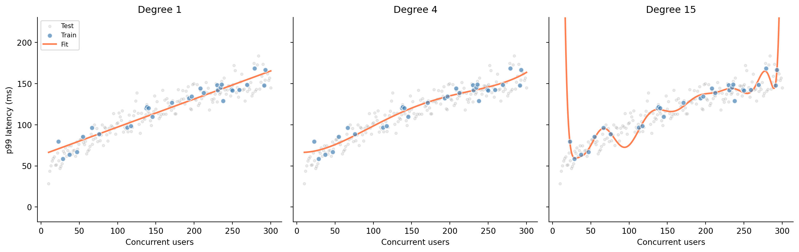
You're building a latency model: given the number of concurrent users hitting a service, predict the p99 response time. You have 30 observations from a load test. The true relationship is smooth (response time grows roughly as the square root of concurrency) but your data is noisy. How flexible should your model be?
```{python}
#| label: fig-polynomial-overfit
#| echo: true
#| fig-cap: "Three polynomial fits to the same data. Degree 1 underfits (misses the curve), degree 4 captures the trend, and degree 15 memorises the training data — including its noise."
#| fig-alt: "Three scatter plots side by side sharing the same axes. Each shows 30 training points in blue and 200 test points in grey. Left panel: a straight line that misses the curve in the data. Centre panel: a smooth degree-4 polynomial that follows the trend. Right panel: a wildly oscillating degree-15 polynomial that passes through every training point but swings far from the test data between them."
rng = np.random.default_rng(42)

# True relationship: p99 latency grows as sqrt of concurrent users
x_train = np.sort(rng.uniform(10, 300, 30))
y_train = 20 + 8 * np.sqrt(x_train) + rng.normal(0, 10, 30)

x_test = np.linspace(10, 300, 200)
y_test = 20 + 8 * np.sqrt(x_test) + rng.normal(0, 10, 200)

x_smooth = np.linspace(10, 300, 500)

fig, axes = plt.subplots(1, 3, figsize=(14, 4.5), sharey=True)
fig.patch.set_alpha(0)
for ax in axes:
    ax.patch.set_alpha(0)

for ax, degree in zip(axes, [1, 4, 15]):
    ax.scatter(x_test, y_test, alpha=0.15, color='grey', s=10, label='Test')
    ax.scatter(x_train, y_train, alpha=0.7, color='#0072B2',
               edgecolor='white', zorder=3, label='Train')

    # Fit a degree-d polynomial and evaluate it
    coeffs = np.polyfit(x_train, y_train, degree)
    y_smooth = np.polyval(coeffs, x_smooth)
    ax.plot(x_smooth, y_smooth, color='#E69F00', linewidth=2, label='Fit')

    ax.set_title(f'Degree {degree}')
    ax.set_xlabel('Concurrent users')
    if degree == 1:
        ax.set_ylabel('p99 latency (ms)')
    ax.spines[['top', 'right']].set_visible(False)

# Clip y-axis to data range so degree-15 oscillations don't crush other panels
y_margin = 0.3 * (y_test.max() - y_test.min())
axes[0].set_ylim(y_test.min() - y_margin, y_test.max() + y_margin)

axes[0].legend(loc='upper left', fontsize=8)
plt.tight_layout()
plt.show()
```
The degree-15 polynomial hits every training point almost exactly: its training error is near zero. But look at how it behaves between and beyond those points: wild oscillations that bear no resemblance to the underlying relationship. It has memorised the training data, noise and all, rather than learning the signal. In @sec-regression-prediction we split data into training and test sets, and warned that a model performing well only on its training data is useless. Now you can see why.
```{python}
#| label: fig-train-test-error
#| echo: true
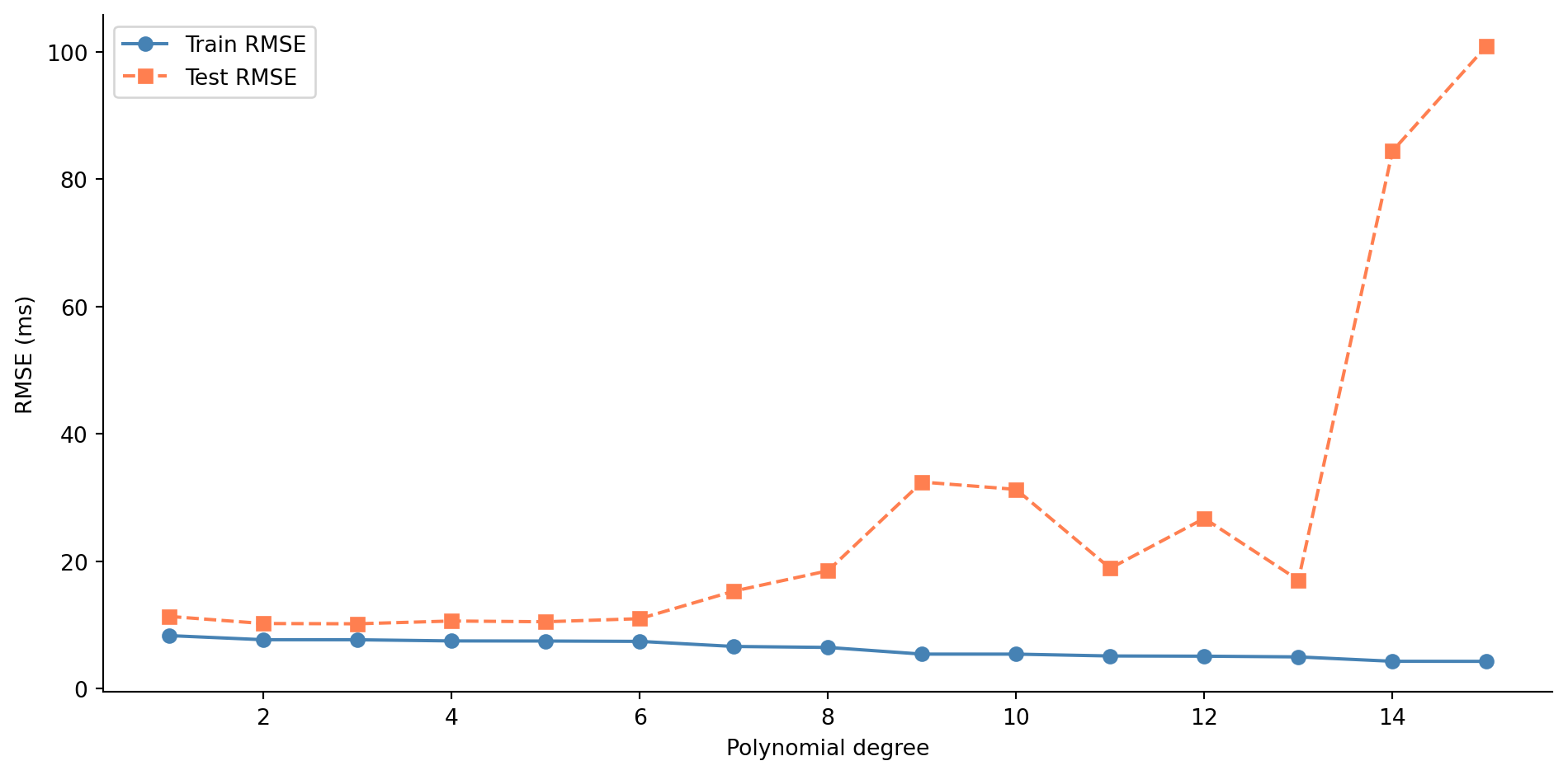
#| fig-cap: "Train and test RMSE across polynomial degrees 1–15. Training error falls monotonically, but test error rises sharply beyond the low degrees — the classic signature of overfitting."
#| fig-alt: "Line chart with polynomial degree on the horizontal axis and RMSE on the vertical axis. The blue training error line with circle markers decreases steadily from left to right. The orange test error line with square markers decreases until around degree 3–4, then rises sharply, forming a U-shape. The gap between the two lines widens as model complexity increases."
from sklearn.metrics import root_mean_squared_error

degrees = range(1, 16)
train_errors, test_errors = [], []

for d in degrees:
    coeffs = np.polyfit(x_train, y_train, d)
    train_errors.append(root_mean_squared_error(y_train, np.polyval(coeffs, x_train)))
    test_errors.append(root_mean_squared_error(y_test, np.polyval(coeffs, x_test)))

fig, ax = plt.subplots(figsize=(10, 5))
fig.patch.set_alpha(0)
ax.patch.set_alpha(0)
ax.plot(list(degrees), train_errors, 'o-', color='#0072B2', label='Train RMSE')
ax.plot(list(degrees), test_errors, 's--', color='#E69F00', label='Test RMSE')
ax.set_title('Test error is U-shaped: complexity past the optimum hurts')
ax.set_xlabel('Polynomial degree')
ax.set_ylabel('RMSE (ms)')
ax.legend()
ax.spines[['top', 'right']].set_visible(False)
plt.tight_layout()
plt.show()
```
@fig-train-test-error shows the classic overfitting signature. Training error decreases as you add flexibility, because more parameters can always fit the training data more closely. But test error follows a U-shape: it improves as the model captures real structure, then worsens as it starts fitting noise. The gap between the two curves is the heart of the problem. A model's value lies in how it performs on data it hasn't seen, not in how well it memorises data it has.
## The bias-variance trade-off {#sec-bias-variance}
This U-shaped test error curve reflects a fundamental tension in predictive modelling. **Bias** is the systematic error: the gap between the model's average prediction (across different training samples) and the truth. A straight line fit to a curved relationship has high bias: no matter how much data you give it, it will systematically miss the curve. **Variance** is the instability: how much the model's predictions change when you train it on a different sample. The degree-15 polynomial has high variance: train it on a slightly different set of 30 points and you get a wildly different curve. **Irreducible error** is the randomness inherent in the data-generating process, the variance of the $\varepsilon$ from @sec-dgp. No model can eliminate it.
For any model evaluated with squared error, the expected test error decomposes into these three components:
$$
\mathbb{E}[\text{test error}] = \text{Bias}^2 + \text{Variance} + \text{Irreducible error}
$$
This decomposition is specific to squared error loss. Under other loss functions (like log-loss for classification), the decomposition takes a more complex form, but the core intuition holds: simple models underfit, complex models overfit, and the best test-set performance lies somewhere in between.
::: {.callout-note}
## Engineering Bridge
Think of bias as a systematic miscalibration, like a monitoring dashboard that consistently underreports latency by 10%. It's wrong in a *predictable* way. Variance is flakiness — like a test that passes 60% of the time, with results that depend on which data happened to be in the cache. You'd rather have a dashboard that's reliably off by a small amount (low variance, moderate bias) than one that's sometimes perfect and sometimes wildly wrong (low bias, high variance). Regularisation is the technique for trading a small amount of bias for a large reduction in variance.
:::
::: {.callout-tip}
## Author's Note
The idea that deliberately accepting systematic error, bias, is a rational strategy for building better models runs against every engineering instinct. Engineering culture treats bugs as failures to be eliminated; the whole discipline is oriented towards correctness. Yet the bias-variance trade-off says something stranger: that a model which is *reliably wrong in a small, predictable way* can outperform one that is *sometimes right but unpredictably so*. Stability bought through deliberate constraint is a feature, not a compromise.
The test-case analogy helps: an implementation that special-cases every edge case in the test suite will pass those tests perfectly but fail on inputs it hasn't seen. A simpler, more principled implementation may not pass every edge case, but it generalises. The special-cased version has zero training error and high variance; the principled version has small bias and low variance. Regularisation is the mechanism for choosing the latter deliberately, rather than hoping the training data was representative enough to make the former work.
:::
## Penalising complexity {#sec-penalty-idea}
Regularisation addresses the bias-variance trade-off systematically: instead of just minimising the training error, we penalise the model for being too complex. The modified objective becomes:
$$
\text{Loss} = \underbrace{\sum_{i=1}^{n}(y_i - \hat{y}_i)^2}_{\text{RSS}} + \alpha \cdot \text{penalty}(\boldsymbol{\beta})
$$
where $\boldsymbol{\beta}$ is the vector of model coefficients (the $\beta_1, \ldots, \beta_p$ from @sec-multiple-regression, with $p$ the number of features) and $\alpha$ controls the strength of the penalty. (Yes, $\alpha$ is the same letter we used for the significance level in @sec-testing-framework; here it means something entirely different. Scikit-learn uses `alpha` for the regularisation parameter, so we follow that convention; just be aware that the two $\alpha$s have nothing to do with each other.) When $\alpha = 0$, you get ordinary least squares with no constraint on the coefficients. As $\alpha$ increases, the model is forced to keep its coefficients small, which limits its ability to fit noise. The intercept $\beta_0$ is not penalised: we don't want to constrain the model's baseline prediction, only the influence of individual features.
Let's set up a scenario where this matters. You're modelling CI build duration from build metrics: 200 observations with 20 features. Five of those features genuinely affect build time; the other 15 are noise (metrics that were logged but have no predictive value).
```{python}
#| label: build-metrics-setup
#| echo: true
#| code-fold: true
#| code-summary: "Expand to see data-generation code"
from sklearn.model_selection import train_test_split
from sklearn.linear_model import LinearRegression

rng = np.random.default_rng(42)
n = 200

# 5 informative features
files_changed = rng.uniform(5, 80, n)
test_count = rng.uniform(50, 500, n)
cyclomatic_complexity = rng.uniform(1, 20, n)
dependency_depth = rng.uniform(1, 8, n)
cache_hit_rate = rng.uniform(0, 1, n)

# 15 noise features
noise_features = rng.normal(0, 1, (n, 15))

# True relationship: only the 5 real features matter
build_duration = (
    120
    + 2.5 * files_changed
    + 0.4 * test_count
    + 1.8 * cyclomatic_complexity
    + 8.0 * dependency_depth
    - 60.0 * cache_hit_rate  # a warm cache shaves up to ~60s off the build
    + rng.normal(0, 25, n)
)

# Combine into a DataFrame
informative_names = ['files_changed', 'test_count', 'cyclomatic_complexity',
                     'dependency_depth', 'cache_hit_rate']
noise_names = [f'metric_{i}' for i in range(15)]

X = pd.DataFrame(
    np.column_stack([files_changed, test_count, cyclomatic_complexity,
                     dependency_depth, cache_hit_rate, noise_features]),
    columns=informative_names + noise_names
)
y = pd.Series(build_duration, name='build_duration')

X_train, X_test, y_train, y_test = train_test_split(
    X, y, test_size=0.3, random_state=42
)
```
```{python}
#| label: ols-baseline
#| echo: true
# OLS baseline
ols = LinearRegression().fit(X_train, y_train)
print(f"OLS — Train RMSE: {root_mean_squared_error(y_train, ols.predict(X_train)):.1f}s")
print(f"OLS — Test  RMSE: {root_mean_squared_error(y_test, ols.predict(X_test)):.1f}s")
```
OLS fits every coefficient it can, including those 15 noise features. Each one picks up a bit of random correlation in the training data, and those spurious patterns don't generalise. The gap between train and test RMSE tells the story.
## Ridge regression: shrinking coefficients {#sec-ridge}
**Ridge regression** adds an L2 penalty, the sum of squared coefficients, to the loss function. Formally:
$$
\text{Loss}_{\text{ridge}} = \sum_{i=1}^{n}(y_i - \hat{y}_i)^2 + \alpha \sum_{j=1}^{p} \beta_j^2
$$
Scikit-learn's `Ridge` uses exactly this formulation, with the parameter called `alpha`. (The mathematical literature often uses $\lambda$ for the same quantity; we'll use $\alpha$ throughout to match the code.) The penalty discourages large coefficients. Features that contribute real signal retain substantial coefficients because the RSS reduction outweighs the penalty. Features that contribute only noise see their coefficients shrink towards zero; the penalty cost exceeds the marginal training-error reduction.
A critical preprocessing step: because the penalty applies equally to all coefficients, features must be on the same scale. If `test_count` ranges from 50 to 500 while `cache_hit_rate` ranges from 0 to 1, unscaled coefficients would be penalised unevenly. **StandardScaler** centres each feature to mean 0 and scales it to standard deviation 1. Crucially, we fit the scaler on the training data only, then apply that same transformation to the test data; leaking test-set statistics into the scaler would contaminate the evaluation. In production, you'd wrap the scaler and the model in a `sklearn.pipeline.Pipeline` to ensure they always travel together, the same encapsulation instinct you'd apply to any stateful component.
```{python}
#| label: fig-ridge-path
#| echo: true
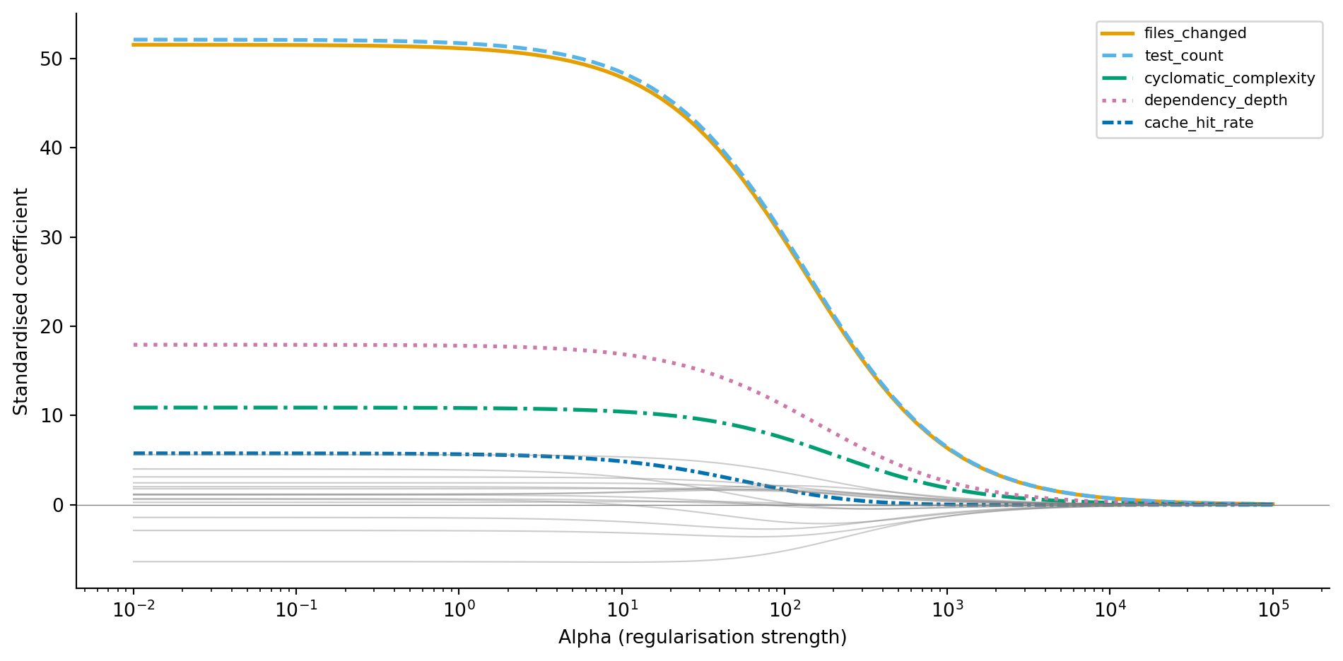
#| fig-cap: "Ridge coefficient paths as regularisation increases. Informative features (coloured, with distinct line styles) retain larger coefficients while noise features (grey) shrink towards zero."
#| fig-alt: "Line chart with log alpha on the horizontal axis and standardised coefficient value on the vertical axis. Five lines with distinct colours and line styles represent informative features: files_changed, test_count, cyclomatic_complexity, dependency_depth, and cache_hit_rate. These maintain distinct non-zero values across a wide range of alpha, with files_changed and test_count retaining the largest magnitudes. Fifteen grey lines representing noise features cluster near zero and shrink further as alpha increases."
from sklearn.preprocessing import StandardScaler
from sklearn.linear_model import Ridge

scaler = StandardScaler()
X_train_scaled = scaler.fit_transform(X_train)
X_test_scaled = scaler.transform(X_test)

alphas = np.logspace(-2, 5, 100)
ridge_coefs = []

for a in alphas:
    ridge = Ridge(alpha=a)
    ridge.fit(X_train_scaled, y_train)
    ridge_coefs.append(ridge.coef_)

ridge_coefs = np.array(ridge_coefs)

fig, ax = plt.subplots(figsize=(10, 5))
fig.patch.set_alpha(0)
ax.patch.set_alpha(0)

# Colour-blind safe palette (Okabe-Ito) with distinct line styles
cb_colours = ['#0072B2', '#E69F00', '#009E73', '#D55E00', '#56B4E9']
cb_styles = ['-', '--', '-.', ':', (0, (3, 1, 1, 1))]

for j, (name, colour, style) in enumerate(zip(informative_names, cb_colours, cb_styles)):
    ax.plot(alphas, ridge_coefs[:, j], color=colour, linewidth=2,
            linestyle=style, label=name)

for j in range(5, 20):
    ax.plot(alphas, ridge_coefs[:, j], color='grey', alpha=0.4, linewidth=0.8)

ax.set_xscale('log')
ax.set_title('Ridge shrinks every coefficient but zeros none')
ax.set_xlabel('Alpha (regularisation strength)')
ax.set_ylabel('Standardised coefficient')
ax.legend(loc='upper right', fontsize=8)
ax.axhline(0, color='grey', linewidth=0.5)
ax.spines[['top', 'right']].set_visible(False)
plt.tight_layout()
plt.show()
```
@fig-ridge-path tells a clear story. At low alpha (left), coefficients are large and noisy, close to OLS. As alpha increases, all coefficients shrink, but the informative features resist the pull towards zero because they genuinely reduce the training error. The noise features (grey) collapse towards zero quickly because their contribution to RSS reduction was spurious. Ridge has a closed-form solution (the OLS normal equations with a modified matrix), so fitting is fast even for large datasets.
::: {.callout-note}
## Engineering Bridge
Regularisation is resource throttling for models. Just as you'd set CPU limits on microservices to prevent any single service from monopolising the cluster, Ridge constrains every coefficient to prevent any single feature from dominating the model unchecked. Every feature still runs — none is shut down — but none can consume unbounded capacity. The penalty parameter $\alpha$ controls how tight the quota is: too loose and a noisy feature can hog the model's expressive power (over-engineering); too tight and genuinely useful features can't do their work (over-simplification).
:::
## Lasso regression: shrinking and selecting {#sec-lasso}
**Lasso regression** replaces the squared penalty with an absolute-value penalty, the L1 norm:
$$
\text{Loss}_{\text{lasso}} = \frac{1}{2n}\sum_{i=1}^{n}(y_i - \hat{y}_i)^2 + \alpha \sum_{j=1}^{p} |\beta_j|
$$
Note the $1/(2n)$ normalisation of the RSS term: this is how scikit-learn's `Lasso` is parameterised, and it means that alpha values for Lasso and Ridge are *not* directly comparable. (Ridge uses the unnormalised RSS.) Lasso's optimal alpha is often smaller than Ridge's, but the important point is that the two live on different scales — comparing their numerical values directly tells you nothing.
This seemingly small change from L2 to L1 has a striking consequence: Lasso can drive coefficients exactly to zero. Where Ridge shrinks coefficients *towards* zero but never quite reaches it, Lasso *eliminates* features entirely. This makes Lasso a feature selection method as well as a regularisation method. Unlike Ridge, which has a closed-form solution, Lasso requires an iterative algorithm called coordinate descent (hence the `max_iter` parameter in the code below) because the L1 penalty is not differentiable at zero.
The mathematical reason for sparsity is geometric. The L1 penalty creates a diamond-shaped constraint region in coefficient space, and the optimal solution tends to land at a corner of that diamond, where one or more coordinates are exactly zero. The L2 penalty creates a circular constraint region with no corners, so the solution slides along the surface without hitting zero.
```{python}
#| label: fig-lasso-path
#| echo: true
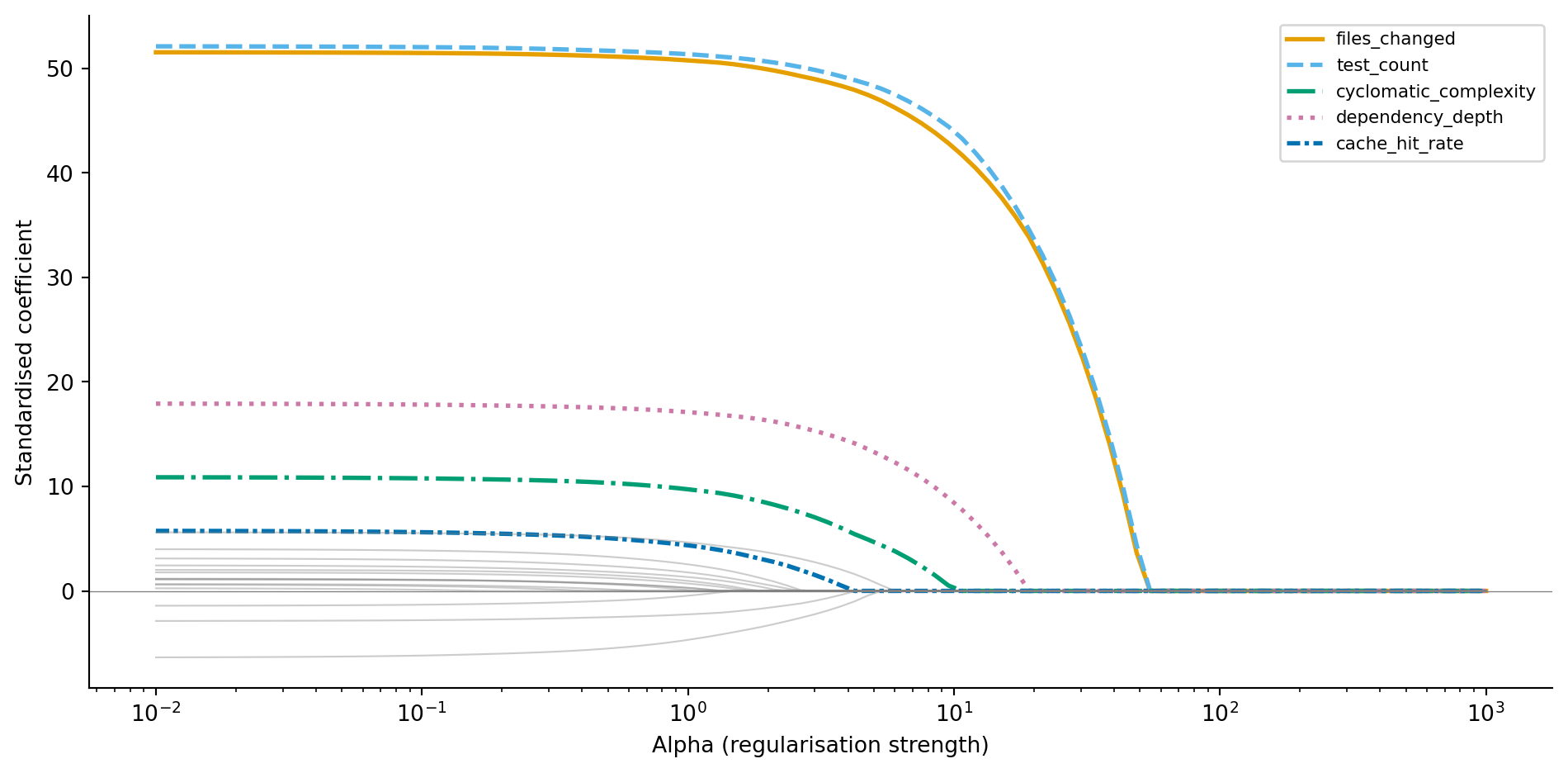
#| fig-cap: "Lasso coefficient paths. Unlike Ridge, coefficients hit exactly zero as alpha increases — noise features are eliminated first, followed by weaker informative features."
#| fig-alt: "Line chart with log alpha on the horizontal axis and standardised coefficient value on the vertical axis. Five lines with distinct colours and line styles represent informative features: files_changed, test_count, cyclomatic_complexity, dependency_depth, and cache_hit_rate. These maintain non-zero values over a wide range before eventually reaching zero at high alpha. Fifteen grey lines representing noise features hit zero much earlier, showing that Lasso performs feature selection by eliminating irrelevant features first."
from sklearn.linear_model import Lasso

lasso_coefs = []
lasso_alphas = np.logspace(-2, 3, 100)

for a in lasso_alphas:
    lasso = Lasso(alpha=a, max_iter=10_000)
    lasso.fit(X_train_scaled, y_train)
    lasso_coefs.append(lasso.coef_)

lasso_coefs = np.array(lasso_coefs)

fig, ax = plt.subplots(figsize=(10, 5))
fig.patch.set_alpha(0)
ax.patch.set_alpha(0)

for j, (name, colour, style) in enumerate(zip(informative_names, cb_colours, cb_styles)):
    ax.plot(lasso_alphas, lasso_coefs[:, j], color=colour, linewidth=2,
            linestyle=style, label=name)

for j in range(5, 20):
    ax.plot(lasso_alphas, lasso_coefs[:, j], color='grey', alpha=0.4, linewidth=0.8)

ax.set_xscale('log')
ax.set_title('Lasso drives noise features to exactly zero')
ax.set_xlabel('Alpha (regularisation strength)')
ax.set_ylabel('Standardised coefficient')
ax.legend(loc='upper right', fontsize=8)
ax.axhline(0, color='grey', linewidth=0.5)
ax.spines[['top', 'right']].set_visible(False)
plt.tight_layout()
plt.show()
```
Compare @fig-lasso-path to @fig-ridge-path. The noise features don't just shrink towards zero — they *become* zero. At higher alpha values, Lasso eliminates noise features entirely while the informative features persist. Let's use cross-validated Lasso to find the optimal alpha and see which features survive.
```{python}
#| label: lasso-selected-features
#| echo: true
from sklearn.linear_model import LassoCV

lasso_cv = LassoCV(cv=5, random_state=42, max_iter=10_000)
lasso_cv.fit(X_train_scaled, y_train)

coef_df = pd.DataFrame({
    'feature': informative_names + noise_names,
    'coefficient': lasso_cv.coef_
}).sort_values('coefficient', key=abs, ascending=False)

print(f"Optimal alpha: {lasso_cv.alpha_:.4f}\n")
print('Non-zero coefficients:')
print(coef_df[coef_df['coefficient'] != 0].to_string(index=False))
print(f"\nFeatures eliminated: {(coef_df['coefficient'] == 0).sum()} of 20")
```
LassoCV selects the alpha that minimises cross-validated prediction error, not the alpha that produces the sparsest model. At this optimal alpha, all five informative features survive, and every one of them ends up with a larger coefficient than any of the noise features. But most of the noise features are retained too, with small non-zero coefficients: because LassoCV tunes alpha for prediction accuracy rather than sparsity, it tolerates a scattering of tiny noise coefficients whenever they nudge cross-validated error down. The coefficient path above shows the alternative — push alpha higher and those noise coefficients drop to zero one by one. If you want a genuinely sparse model, increase alpha beyond the CV-optimal value, trading a little prediction accuracy for simplicity.
::: {.callout-note}
## Engineering Bridge
If Ridge is resource throttling, Lasso is dependency pruning. Ridge keeps every feature but limits its influence. Lasso removes features entirely — like running a dependency audit and stripping out packages your codebase doesn't actually import. The result is a simpler model that's easier to understand, cheaper to compute, and less likely to break when the input distribution shifts. In a production ML system, fewer features also means fewer data pipelines to maintain, fewer points of failure, and a smaller attack surface for data quality issues.
:::
## Elastic Net: combining L1 and L2 {#sec-elastic-net}
**Elastic Net** blends both penalties:
$$
\text{Loss}_{\text{elastic}} = \frac{1}{2n}\sum_{i=1}^{n}(y_i - \hat{y}_i)^2 + \alpha \left[ \rho \sum_{j=1}^{p} |\beta_j| + \frac{1 - \rho}{2} \sum_{j=1}^{p} \beta_j^2 \right]
$$
where $\rho$ (scikit-learn's `l1_ratio` parameter) controls the mix between L1 and L2. When $\rho = 1$, it's pure Lasso; when $\rho = 0$, it's pure Ridge.
Why bother with a hybrid? Lasso has a weakness: when features are correlated with each other, it tends to arbitrarily pick one feature from a correlated group and zero out the others. Which feature it picks can change with a different training sample, making the model unstable. Elastic Net's L2 component encourages the model to spread the coefficient across the correlated group, producing more stable and reproducible results. The trade-off is that you now have two hyperparameters to tune ($\alpha$ and $\rho$), and `ElasticNetCV` can search over both simultaneously: supply a list of candidate `l1_ratio` values along with the cross-validation folds, and it evaluates all combinations to find the pair that minimises prediction error.
```{python}
#| label: elastic-net-demo
#| echo: true
from sklearn.linear_model import ElasticNetCV

elastic_cv = ElasticNetCV(
    l1_ratio=[0.1, 0.5, 0.7, 0.9, 0.95, 0.99],
    cv=5, random_state=42, max_iter=10_000
)
elastic_cv.fit(X_train_scaled, y_train)

n_nonzero = np.sum(elastic_cv.coef_ != 0)
print(f"Elastic Net — alpha: {elastic_cv.alpha_:.4f}, "
      f"l1_ratio: {elastic_cv.l1_ratio_:.2f}")
print(f"Non-zero coefficients: {n_nonzero} of 20")
print(f"Test RMSE: {root_mean_squared_error(y_test, elastic_cv.predict(X_test_scaled)):.1f}s")
```
## Choosing the regularisation strength {#sec-choosing-alpha}
The regularisation strength $\alpha$ is a **hyperparameter**: a setting you choose before fitting, not a value the model learns from data. Too low and you don't prevent overfitting; too high and you squash genuine signal. How do you find the right value?
**Cross-validation** provides the answer. Instead of a single train/test split, you divide the training data into $k$ approximately equally sized **folds** (typically 5 or 10). For each candidate $\alpha$, you train the model $k$ times, each time holding out a different fold for evaluation. The $\alpha$ that produces the lowest average error across all $k$ folds wins.
Scikit-learn's `RidgeCV`, `LassoCV`, and `ElasticNetCV` handle this automatically. You supply a grid of candidate alphas (or let the library choose sensible defaults), and the `*CV` estimator evaluates each one using $k$-fold cross-validation, then refits the model on the full training set using the winning alpha.
```{python}
#| label: fig-model-comparison
#| echo: true
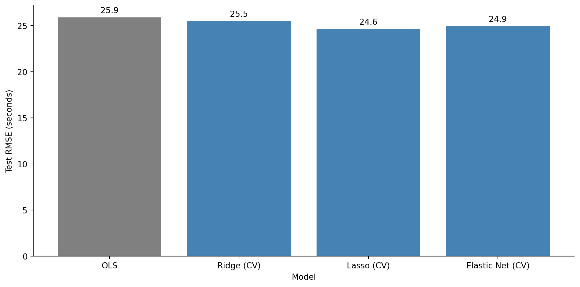
#| fig-cap: "Test RMSE for OLS versus regularised models with cross-validated alpha. All three regularised variants outperform unregularised OLS."
#| fig-alt: "Bar chart comparing test RMSE in seconds for OLS, Ridge (CV), Lasso (CV), and Elastic Net (CV). The OLS bar in grey is the tallest. The three regularised model bars in blue are shorter and roughly similar in height. RMSE values are labelled above each bar."
from sklearn.linear_model import RidgeCV

ridge_cv = RidgeCV(alphas=np.logspace(-2, 5, 100), cv=5)
ridge_cv.fit(X_train_scaled, y_train)

# Each model predicts using the data representation it was trained on:
# OLS was fit on unscaled data, regularised models on scaled data.
models = {
    'OLS': ols.predict(X_test),
    'Ridge (CV)': ridge_cv.predict(X_test_scaled),
    'Lasso (CV)': lasso_cv.predict(X_test_scaled),
    'Elastic Net (CV)': elastic_cv.predict(X_test_scaled),
}

fig, ax = plt.subplots(figsize=(10, 5))
fig.patch.set_alpha(0)
ax.patch.set_alpha(0)
names = list(models.keys())
rmses = [root_mean_squared_error(y_test, preds) for preds in models.values()]
bar_colours = ['grey', '#0072B2', '#0072B2', '#0072B2']
bars = ax.bar(names, rmses, color=bar_colours, edgecolor='none')

for bar, rmse in zip(bars, rmses):
    ax.text(bar.get_x() + bar.get_width() / 2, bar.get_height() + 0.3,
            f'{rmse:.1f}', ha='center', va='bottom', fontsize=10)

ax.set_title('Regularised models beat unregularised OLS on the test set')
ax.set_xlabel('Model')
ax.set_ylabel('Test RMSE (seconds)')
ax.spines[['top', 'right']].set_visible(False)
plt.tight_layout()
plt.show()

print(f"Ridge α:       {ridge_cv.alpha_:.2f}")
print(f"Lasso α:       {lasso_cv.alpha_:.4f}")
print(f"Elastic Net α: {elastic_cv.alpha_:.4f} (l1_ratio={elastic_cv.l1_ratio_:.2f})")
```
All three regularised models outperform OLS on the test set. The noise features that OLS dutifully fitted are now either shrunk (Ridge) or eliminated (Lasso, Elastic Net), and the model generalises better as a result.
::: {.callout-note}
## Engineering Bridge
Cross-validation is the modelling equivalent of parameterised CI testing. Instead of running your test suite against one fixed environment and hoping the results generalise, you run it across multiple configurations: different OS versions, Python versions, dependency sets. Each fold is a different environment. The hyperparameter value that performs consistently well across *all* folds — not just one lucky configuration — is the one you trust. Just as a test that passes on five different OS/Python combinations gives you more confidence than one that passes on a single setup, a cross-validated alpha is more trustworthy than one tuned on a single train/validation split.
:::
## Regularisation in classification {#sec-regularisation-classification}
Everything we've discussed applies to classification too. In @sec-deployment-failure-model, we fitted a `LogisticRegression` and noted in a comment that scikit-learn applies L2 regularisation by default with `C=1.0`. Now you can understand what that means.
Scikit-learn's `C` parameter is the *inverse* of the regularisation strength: $C = 1/\lambda$, where $\lambda$ is the penalty weight. Smaller `C` means stronger regularisation. The default `C=1.0` applies moderate L2 regularisation to every logistic regression you fit with scikit-learn, a sensible default that prevents extreme coefficients but one that can surprise you if you compare the output to an unregularised `statsmodels` fit. This is one of those cases where two libraries parameterise the same concept differently, like `timeout` vs `deadline` semantics in different RPC frameworks.
```{python}
#| label: regularisation-classification
#| echo: true
#| code-fold: true
#| code-summary: "Expand to see deployment data generation (same as Chapter 10)"
from scipy.special import expit
from sklearn.linear_model import LogisticRegression

# Same deployment data from Chapter 10
rng_deploy = np.random.default_rng(42)
n_deploy = 500

deploy_data = pd.DataFrame({
    'files_changed': rng_deploy.integers(1, 80, n_deploy),
    'hours_since_last_deploy': rng_deploy.exponential(24, n_deploy).round(1),
    'is_friday': rng_deploy.binomial(1, 1/5, n_deploy),
    'test_coverage_pct': np.clip(rng_deploy.normal(75, 15, n_deploy), 20, 100).round(1),
})

log_odds = (
    -1.0
    + 0.05 * deploy_data['files_changed']
    + 0.02 * deploy_data['hours_since_last_deploy']
    + 0.8 * deploy_data['is_friday']
    - 0.04 * deploy_data['test_coverage_pct']
)
deploy_data['failed'] = rng_deploy.binomial(1, expit(log_odds))
```
```{python}
#| label: regularisation-classification-comparison
#| echo: true
feature_names = ['files_changed', 'hours_since_last_deploy',
                 'is_friday', 'test_coverage_pct']

# Compare coefficients across regularisation strengths
# (fitting on full data here — we're illustrating coefficient behaviour,
# not evaluating predictive performance)
results = {}
for C in [0.01, 0.1, 1.0, 10.0, 1000.0]:
    clf = LogisticRegression(C=C, max_iter=200, random_state=42)
    clf.fit(deploy_data[feature_names], deploy_data['failed'])
    results[f'C={C}'] = np.append(clf.intercept_, clf.coef_.ravel())

coef_table = pd.DataFrame(results, index=['intercept'] + feature_names).T
print('Logistic regression coefficients at different regularisation strengths:\n')
coef_table.round(4)
```
At `C=0.01` (strong regularisation), all coefficients are heavily shrunk; the model is conservative, barely distinguishing between features. At `C=1000` (near-zero regularisation), the coefficients approach the unregularised values you'd get from `statsmodels`. The default `C=1.0` sits in between, offering a reasonable compromise for most problems.
::: {.callout-tip}
## Author's Note
One of the most disorienting things about the Python data science ecosystem is that different libraries have different defaults for the same concept. Scikit-learn's `LogisticRegression` regularises by default (`C=1.0`); statsmodels doesn't. The parameter is called `C` (the inverse of regularisation strength) rather than `alpha` or `lambda`, which adds another layer of confusion. The coefficients from the two libraries won't match, and the discrepancy looks like a bug until you understand what's happening. The broader lesson: whenever you switch between statistical and ML libraries, check what defaults are silently applied. Sensible defaults are only sensible if you know about them.
:::
## Summary {#sec-regularisation-summary}
1. **Overfitting occurs when a model fits noise in the training data**, producing low training error but poor test-set performance. The classic sign is a growing gap between training and test metrics as complexity increases.
2. **The bias-variance trade-off is fundamental.** Simple models have high bias (systematic error) and low variance (stability); complex models have the reverse. The best test-set performance lies at the balance point.
3. **Ridge (L2) regression shrinks all coefficients towards zero**, reducing variance at the cost of a small increase in bias. It keeps every feature but diminishes the influence of noisy ones.
4. **Lasso (L1) regression drives some coefficients exactly to zero**, performing automatic feature selection. It produces sparser, more interpretable models. Cross-validated Lasso optimises for prediction, not maximal sparsity.
5. **Cross-validation chooses the regularisation strength.** Splitting the training data into folds and evaluating each candidate $\alpha$ prevents you from overfitting the hyperparameter to one particular split.
## Exercises {#sec-regularisation-exercises}
1. Using the same `x_train` and `y_train` from @fig-polynomial-overfit, fit polynomial features of degree 15 using `sklearn.preprocessing.PolynomialFeatures` (with `include_bias=False`), then apply Ridge regression with `RidgeCV`. Compare the resulting curve to the unregularised degree-15 fit. Does Ridge tame the oscillations? (*Hint:* degree-15 polynomial features span an enormous range of magnitudes — feature 1 runs from 10 to 300 but feature 15 runs from $10^{15}$ to $300^{15}$. Use a `Pipeline` that applies `PolynomialFeatures` and then `StandardScaler` (scaling the expanded features) to avoid numerical instability.)
2. **Feature selection comparison.** Generate a dataset with 50 features (10 informative, 40 noise) and 150 observations. Fit OLS, Ridge, and Lasso. For each model, count how many noise features have coefficients larger than 0.1 in absolute value. Which method best separates signal from noise?
3. **Conceptual:** Explain why features must be standardised before applying Ridge or Lasso, but not before fitting ordinary least squares. What would happen if you applied Lasso to unstandardised features where one feature ranges from 0 to 1 and another from 0 to 1,000,000?
4. **Regularisation strength for classification.** Recreate the deployment failure model from @sec-deployment-failure-model. Fit `LogisticRegression` with `C` values of 0.001, 0.01, 0.1, 1.0, 10.0, and 100.0. For each, compute the test-set AUC. Plot AUC vs $\log_{10}(C)$. At what point does reducing regularisation stop helping?
5. **Conceptual:** A colleague says "I always use Lasso because it selects features for me, so it's strictly better than Ridge." Give two scenarios where Ridge would be the better choice. (*Hint:* think about correlated features and what "better" means when interpretability isn't the goal.)
6. **Conceptual:** The chapter likens Lasso to dependency pruning — stripping out the features a model doesn't really use, the way you'd remove unused packages from a project. Where does that analogy break down? Consider how each decides what to drop, how stable that decision is across different samples or correlated inputs, and whether dropping something the method deems unimportant is as consequence-free as removing an unused import.