16  Reproducible data science

16.1 The build that works on your machine

Every software engineer has heard it: “It works on my machine.” We’ve spent decades building infrastructure to eliminate that phrase — deterministic build systems, pinned dependencies, containerised deployments, infrastructure as code. When you push code to main, CI rebuilds the entire artefact from scratch, and if the output differs from what you tested locally, something is wrong.

Data science has the same problem, magnified. A model trained on your laptop produces different results on a colleague’s machine — not because the code is wrong, but because the NumPy version differs, or the random seed propagated differently across threads, or the training data was filtered using a query that returned different rows after yesterday’s ETL job updated the source table. The code is identical. The output is not.

This matters more than it might seem. A model that can’t be reproduced can’t be audited, can’t be debugged, and can’t be trusted. When a stakeholder asks “why did the model flag this transaction as fraud?” and you can’t reconstruct the model that made that decision, you have a governance problem, not just an engineering one.

The good news: everything you know about making software reproducible applies here. The bad news: data science introduces several new dimensions of variability that software builds don’t have. This chapter maps out those dimensions and gives you practical tools to control them.

16.2 The four layers of reproducibility

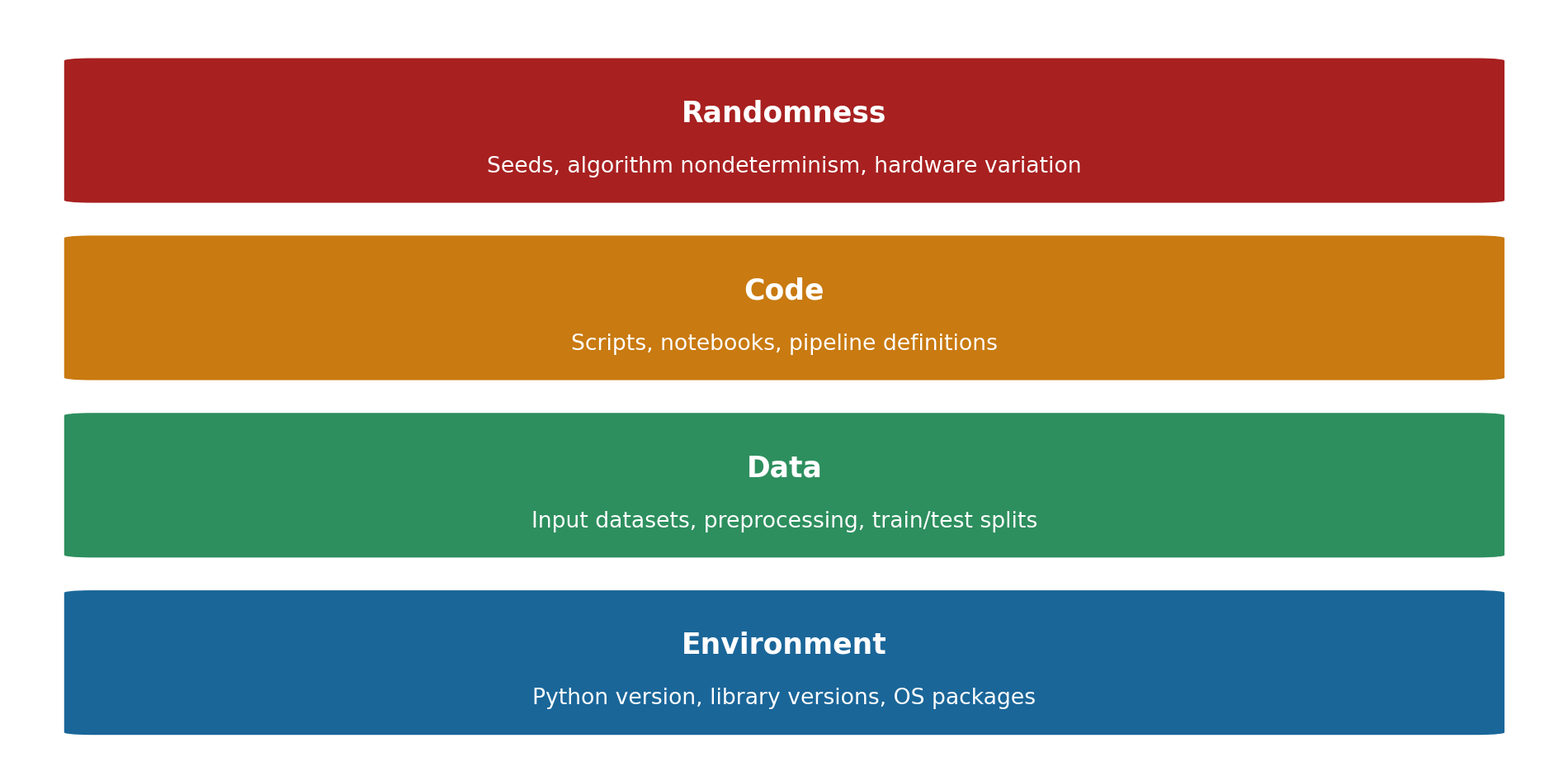
A software build is reproducible when the same source code produces the same binary. A data science result is reproducible when the same code, run on the same data, with the same environment, produces the same output. That’s three more things to pin down than a typical software project.

We can organise these into four layers, each building on the last (Figure 16.1).

import matplotlib.pyplot as plt
import matplotlib.patches as mpatches

fig, ax = plt.subplots(figsize=(10, 5))

layers = [
    ("Environment", "Python version, library versions, OS packages", "#1a6699"),
    ("Data", "Input datasets, preprocessing, train/test splits", "#2d8f5e"),
    ("Code", "Scripts, notebooks, pipeline definitions", "#c97a10"),
    ("Randomness", "Seeds, algorithm nondeterminism, hardware variation", "#a82020"),
]

y = 0
for label, desc, colour in layers:
    rect = mpatches.FancyBboxPatch(
        (0.05, y + 0.05), 0.9, 0.8,
        boxstyle="round,pad=0.02", facecolor=colour,
        edgecolor='white', linewidth=2
    )
    ax.add_patch(rect)
    ax.text(0.5, y + 0.55, label, ha='center', va='center',
            fontsize=13, fontweight='bold', color='white')
    ax.text(0.5, y + 0.25, desc, ha='center', va='center',
            fontsize=10, color='white')
    y += 1

ax.set_xlim(0, 1)
ax.set_ylim(-0.1, 4.1)
ax.axis('off')
fig.tight_layout()
plt.show()

Figure 16.1: The four layers of data science reproducibility. Each layer depends on the ones below it.

In software engineering, the environment layer is largely solved (Docker, Nix, lock files). The data layer doesn’t usually exist — your build inputs are source files checked into version control. The code layer is the only one that matters, and git handles it. The randomness layer is irrelevant for deterministic programs.

Data science needs all four.

16.3 Environment reproducibility

You already know how to pin dependencies. The difference in data science is that the dependency tree is deeper and more fragile. NumPy, SciPy, and scikit-learn all wrap compiled C, C++, and Fortran libraries (BLAS and LAPACK — the low-level linear algebra libraries that NumPy delegates to). A minor version bump in any of these can change numerical results — not because of bugs, but because of legitimate improvements to floating-point algorithms or different library implementations.

A requirements.txt with loose pins isn’t enough:

# This is insufficient for reproducibility
numpy>=1.26    # could resolve to 1.26.0 today, 1.26.4 next month
scikit-learn   # completely unpinned

Exact pins are better. A lock file is best:

# requirements.lock — generated by pip-compile, pip freeze, or similar
numpy==1.26.4
scikit-learn==1.4.2
scipy==1.12.0
joblib==1.3.2       # transitive dependency of scikit-learn

Tools like pip-compile (from pip-tools), poetry.lock, or uv.lock generate these automatically. They resolve the full dependency graph and pin every package — including transitive dependencies that you never explicitly asked for but that can still change your results.

Engineering Bridge

If you’ve used package-lock.json in Node.js or Cargo.lock in Rust, this is the same idea. The difference is that in web development, a lock file mainly prevents “it broke in production because a dependency updated.” In data science, a lock file also prevents “the model produces different predictions because a dependency updated.” The failure mode is silent — your pipeline runs without errors but produces subtly different numbers — which makes it harder to detect and more dangerous than a crash.

For full environment isolation, containers are the standard approach. A Dockerfile pins the OS, system libraries, Python version, and all packages in one reproducible unit:

# Dockerfile for a reproducible training environment
FROM python:3.11.8-slim

COPY requirements.lock /app/requirements.lock
RUN pip install --no-cache-dir -r /app/requirements.lock

COPY src/ /app/src/
WORKDIR /app

If you’ve containerised a web service, the Dockerfile structure will feel familiar. The additional data-science-specific consideration is that some packages (particularly those using GPU acceleration) need specific system-level libraries — CUDA drivers, OpenBLAS, MKL — that must also be pinned in the container.

16.4 Data reproducibility

This is the layer that software engineering doesn’t prepare you for. Your training data are inputs to the model just as surely as your source code, but they don’t fit neatly into git. Datasets can be gigabytes or terabytes. They change over time as new records arrive. And the same SQL query can return different results on Monday than it did on Friday.

There are three practical strategies, ranging from simple to sophisticated.

Strategy 1: Snapshot and hash. Save a copy of the exact dataset used for each experiment. Store a content hash (SHA-256) alongside the model artefact so you can verify later that the data hasn’t been tampered with or accidentally swapped.

import hashlib
import pandas as pd
import numpy as np
import io

# Create a sample dataset
rng = np.random.default_rng(42)
df = pd.DataFrame({
    'feature_a': rng.normal(0, 1, 1000),
    'feature_b': rng.uniform(0, 100, 1000),
    'target': rng.binomial(1, 0.3, 1000),
})

def hash_dataframe(df: pd.DataFrame) -> str:
    """Compute a deterministic hash of a DataFrame's contents."""
    buf = io.BytesIO()
    df.to_parquet(buf, index=False)
    return hashlib.sha256(buf.getvalue()).hexdigest()[:16]  # truncated for display

data_hash = hash_dataframe(df)
print(f"Dataset: {df.shape[0]} rows, {df.shape[1]} columns")
print(f"Content hash: {data_hash}")

Dataset: 1000 rows, 3 columns
Content hash: 916a4b2e33326bb6

This is the data equivalent of a git commit hash — a fingerprint that uniquely identifies a specific version of the data. Store it in your experiment metadata, and you can always verify that you’re working with the same data. One caveat: the hash depends on the parquet serialisation library (pyarrow), so the same DataFrame can produce different hashes under different pyarrow versions. Pin your serialisation library alongside the hash, or use a format-independent approach (hashing sorted CSV output) if you need hashes to be stable across library upgrades.

Strategy 2: Data version control. Tools like DVC (Data Version Control) extend git to handle large files. DVC stores the actual data in remote storage (S3, GCS, Azure Blob) and tracks lightweight pointer files in git. Each pointer file contains a hash of the data, so checking out a git commit also checks out the exact data used at that point in time.

# Initialise DVC in an existing git repo
dvc init
dvc remote add -d myremote s3://my-bucket/dvc-store

# Track a dataset
dvc add data/training.parquet
git add data/training.parquet.dvc data/.gitignore
git commit -m "Track training data v1"

# Later, to reproduce: checkout the commit and pull the data
git checkout abc123
dvc pull

Strategy 3: Immutable data stores. For production systems, write each version of a dataset to an immutable location — a timestamped path in object storage, a versioned table in a data warehouse, or a labelled partition. The training pipeline reads from a specific version identifier, never from “latest.”

# Instead of:
df = pd.read_parquet("s3://data-lake/training/features.parquet")

# Use a versioned path:
DATA_VERSION = "2025-01-15T08:00:00"
df = pd.read_parquet(f"s3://data-lake/training/v={DATA_VERSION}/features.parquet")

Author’s Note

Data versioning is the layer that’s easiest to underestimate. Pinning Python dependencies and setting random seeds feels thorough — but if the training data comes from a live database table, the pipeline’s output can change without any code change at all. An upstream data engineering fix, a schema migration, even a backfill can silently alter the training distribution. The model hasn’t improved or degraded — the data has changed underneath it. Treating every dataset like an immutable release artefact is the only reliable defence. If you wouldn’t deploy code from a mutable branch, you shouldn’t train models from a mutable table.

16.5 Taming randomness

Randomness in data science is pervasive and deliberate. Random train/test splits, random weight initialisation, stochastic gradient descent, random feature subsampling in random forests — nearly every step involves drawing from a pseudorandom sequence. Controlling that sequence is straightforward in principle but has several practical traps.

The basic tool is a random seed — a fixed starting point for the pseudorandom number generator (PRNG). We’ve used this throughout the book:

import numpy as np
from sklearn.model_selection import train_test_split
from sklearn.ensemble import RandomForestClassifier

rng = np.random.default_rng(42)

# Generate synthetic data
X = rng.normal(0, 1, (500, 5))
y = (X[:, 0] + 0.5 * X[:, 1] + rng.normal(0, 0.3, 500) > 0).astype(int)

# Reproducible split
X_train, X_test, y_train, y_test = train_test_split(
    X, y, test_size=0.2, random_state=42
)

# Reproducible model training
rf = RandomForestClassifier(n_estimators=100, random_state=42)
rf.fit(X_train, y_train)
print(f"Test accuracy: {rf.score(X_test, y_test):.4f}")

Test accuracy: 0.9200

Run this code twice and you’ll get the same accuracy to the fourth decimal place. But there are three common traps.

Trap 1: Forgetting to seed all sources of randomness. scikit-learn models have their own random_state parameter, train_test_split has another, and if you use NumPy or pandas operations that involve randomness (shuffling, sampling), those draw from yet another PRNG. Missing any one of these introduces variation.

# A disciplined approach: derive all seeds from a single master seed
MASTER_SEED = 42

rng = np.random.default_rng(MASTER_SEED)
split_seed = int(rng.integers(0, 2**31))  # scikit-learn accepts int32 seeds
model_seed = int(rng.integers(0, 2**31))

X_train, X_test, y_train, y_test = train_test_split(
    X, y, test_size=0.2, random_state=split_seed
)

rf = RandomForestClassifier(n_estimators=100, random_state=model_seed)
rf.fit(X_train, y_train)
print(f"Test accuracy (derived seeds): {rf.score(X_test, y_test):.4f}")
print(f"Split seed: {split_seed}, Model seed: {model_seed}")

Test accuracy (derived seeds): 0.8600
Split seed: 191664964, Model seed: 1662057958

A single master seed at the top of your script, with all downstream seeds derived from it, gives you full reproducibility with one number to record.

Trap 2: Parallelism breaks determinism. Many scikit-learn estimators accept an n_jobs parameter for parallel training. When n_jobs > 1, the order of operations depends on thread scheduling, which the operating system controls. The same seed can produce different results depending on how many cores are available and how the OS allocates them.

from sklearn.ensemble import RandomForestClassifier

# Sequential: deterministic
rf_seq = RandomForestClassifier(
    n_estimators=100, random_state=42, n_jobs=1
)
rf_seq.fit(X_train, y_train)
score_seq = rf_seq.score(X_test, y_test)

# Parallel: may vary across runs on different hardware
rf_par = RandomForestClassifier(
    n_estimators=100, random_state=42, n_jobs=-1
)
rf_par.fit(X_train, y_train)
score_par = rf_par.score(X_test, y_test)

print(f"Sequential: {score_seq:.4f}")
print(f"Parallel:   {score_par:.4f}")
print(f"Same result: {score_seq == score_par}")

Sequential: 0.8800
Parallel:   0.8800
Same result: True

For scikit-learn’s random forests specifically, the results are identical because each tree is assigned a deterministic seed before parallel dispatch — there is no shared accumulation across threads. But nondeterminism from parallelism arises in algorithms where threads combine partial results, particularly in GPU-accelerated libraries like XGBoost and LightGBM, where floating-point addition order varies between runs.

Trap 3: Floating-point arithmetic is not associative. In exact arithmetic, \((a + b) + c = a + (b + c)\) — the grouping doesn’t matter. In IEEE 754 floating-point, this is not always true. Different execution orders — caused by different hardware, compiler optimisations, or library versions — can produce results that differ in the last few significant digits. For most analyses this is negligible, but it can compound across thousands of iterations.

import numpy as np

# Demonstrate floating-point non-associativity
a = np.float64(1e-16)
b = np.float64(1.0)
c = np.float64(-1.0)

result_1 = (a + b) + c
result_2 = a + (b + c)

print(f"(a + b) + c = {result_1}")
print(f"a + (b + c) = {result_2}")
print(f"Equal? {result_1 == result_2}")

(a + b) + c = 0.0
a + (b + c) = 1e-16
Equal? False

The practical lesson: aim for bitwise reproducibility on the same hardware and environment, but accept statistical reproducibility (results within a small tolerance) across different platforms. Document which level of reproducibility you guarantee.

Engineering Bridge

This is directly analogous to the distinction between reproducible builds and deterministic builds in software engineering. A reproducible build means anyone can rebuild the artefact from source and get a functionally equivalent result. A deterministic build means the output is bit-for-bit identical. Most CI systems aim for reproducible builds; only security-sensitive contexts (like Debian’s reproducible builds initiative) demand bit-for-bit determinism. Data science has the same spectrum: most workflows should be reproducible to within a small numerical tolerance, while regulated industries (finance, healthcare) may require exact reproducibility.

16.6 Experiment tracking

Software engineers have git log, CI dashboards, and deployment history. The data science equivalent is an experiment tracker — a system that records the parameters, data version, code version, and results of every training run.

Without experiment tracking, the lifecycle of a model looks like this: “I tried a bunch of things last Tuesday, one of them worked, and I think the notebook I used is somewhere in my home directory.” This is the data science equivalent of deploying from a developer’s laptop without version control.

A minimal experiment log needs five fields:

import json
from datetime import datetime, timezone

def log_experiment(params: dict, metrics: dict, data_hash: str,
                   notes: str = "") -> dict:
    """Log an experiment run with full provenance."""
    record = {
        "timestamp": datetime.now(timezone.utc).isoformat(),
        "parameters": params,
        "metrics": metrics,
        "data_hash": data_hash,
        "notes": notes,
    }
    return record

# Example: log the random forest experiment
experiment = log_experiment(
    params={
        "model": "RandomForestClassifier",
        "n_estimators": 100,
        "random_state": 42,
        "test_size": 0.2,
    },
    metrics={
        "test_accuracy": float(rf.score(X_test, y_test)),
        "train_accuracy": float(rf.score(X_train, y_train)),
    },
    data_hash=data_hash,
    notes="Baseline model, all features",
)

print(json.dumps(experiment, indent=2))

{
  "timestamp": "2026-02-18T18:07:57.986756+00:00",
  "parameters": {
    "model": "RandomForestClassifier",
    "n_estimators": 100,
    "random_state": 42,
    "test_size": 0.2
  },
  "metrics": {
    "test_accuracy": 0.86,
    "train_accuracy": 1.0
  },
  "data_hash": "916a4b2e33326bb6",
  "notes": "Baseline model, all features"
}

In practice, dedicated tools handle this at scale. MLflow is the most widely adopted open-source option. It logs parameters, metrics, artefacts (models, plots, data samples), and organises runs into named experiments:

import mlflow

mlflow.set_experiment("churn-prediction")

with mlflow.start_run():
    mlflow.log_param("n_estimators", 100)
    mlflow.log_param("random_state", 42)
    mlflow.log_param("data_hash", data_hash)

    rf = RandomForestClassifier(n_estimators=100, random_state=42)
    rf.fit(X_train, y_train)

    mlflow.log_metric("test_accuracy", rf.score(X_test, y_test))
    mlflow.log_metric("train_accuracy", rf.score(X_train, y_train))
    mlflow.sklearn.log_model(rf, "model")

The structure maps cleanly onto concepts you already know: an experiment is a repository, a run is a commit, parameters are configuration, metrics are test results, and artefacts are build outputs. The difference is that in software, a build either passes or fails; in data science, you’re comparing runs to find the best one among many that all “passed.”

Author’s Note

Experiment tracking feels like overhead — until you try to answer the question “which exact configuration produced the model we deployed?” Manual tracking (spreadsheets, notebook filenames, comments) breaks down as soon as you have more than a handful of runs. The problem isn’t recording the information — it’s recording enough information to distinguish between runs that look nearly identical. “RF, 200 trees, accuracy 0.87” describes dozens of variants with slightly different preprocessing. A proper tracking tool (MLflow, Weights & Biases, even a structured log) captures the full configuration automatically. The setup cost is minutes; the cost of not having it compounds every time you revisit old work.

16.7 From notebooks to pipelines

Jupyter notebooks are excellent for exploration — interactive, visual, immediate. They are poor for reproducibility. The execution order is hidden (cells can be run in any order), state accumulates invisibly (deleting a cell doesn’t delete the variable it created), and notebooks resist diffing, testing, and code review.

This isn’t a reason to abandon notebooks. It’s a reason to treat them as a prototyping environment, not a delivery artefact. The workflow that works in practice is: explore in a notebook, then extract the reproducible pipeline into scripts.

# train.py — extracted from notebook exploration
import argparse
import pandas as pd
from sklearn.ensemble import RandomForestClassifier
from sklearn.model_selection import train_test_split

def main(data_path: str, n_estimators: int, seed: int):
    df = pd.read_parquet(data_path)
    X = df.drop(columns=["target"])
    y = df["target"]
    X_train, X_test, y_train, y_test = train_test_split(
        X, y, test_size=0.2, random_state=seed
    )
    model = RandomForestClassifier(
        n_estimators=n_estimators, random_state=seed
    )
    model.fit(X_train, y_train)
    print(f"Test accuracy: {model.score(X_test, y_test):.4f}")

if __name__ == "__main__":
    parser = argparse.ArgumentParser()
    parser.add_argument("--data", required=True)
    parser.add_argument("--n-estimators", type=int, default=100)
    parser.add_argument("--seed", type=int, default=42)
    args = parser.parse_args()
    main(args.data, args.n_estimators, args.seed)

The script has several properties the notebook lacks: all parameters are explicit arguments (no hidden state), the execution order is unambiguous (top to bottom), it can be called from CI, and it can be reviewed in a pull request with a meaningful diff.

For more complex workflows — where training depends on a preprocessing step, which depends on a data extraction step — pipeline tools encode the dependency graph explicitly. This is the same idea as a build system (Make, Bazel, Gradle), applied to data science:

# dvc.yaml — a DVC pipeline definition (conceptually similar to a Makefile)
stages:
  preprocess:
    cmd: python src/preprocess.py --input data/raw.parquet --output data/features.parquet
    deps:
      - src/preprocess.py
      - data/raw.parquet
    outs:
      - data/features.parquet

  train:
    cmd: python src/train.py --data data/features.parquet --seed 42
    deps:
      - src/train.py
      - data/features.parquet
    params:
      - train.n_estimators
      - train.seed
    outs:
      - models/model.pkl
    metrics:
      - metrics.json:
          cache: false

Each stage declares its inputs (deps), outputs (outs), and the command to run. DVC tracks the hash of every input and output. If you change preprocess.py, DVC knows to re-run preprocessing and training. If you change only train.py, it re-runs training from the cached features. This is dependency-driven execution — the same paradigm as make, but designed for data-heavy workflows.

16.8 Putting it together: a reproducibility checklist

Table 16.1 maps specific practices to each layer. Not every project needs every item, but a production model should satisfy most of them.

Table 16.1: Reproducibility checklist by layer. Essential items are the minimum for any project; production items are recommended for team-maintained systems.

Layer	Essential	Production
Environment	Dependency lock file (pip-compile, uv.lock)	Containerised training environment (Docker)
Data	Snapshot + content hash of training data	Data version control (DVC, immutable stores)
Code	All code in version control (no final_v3_REAL.ipynb)	Pipeline orchestration (DVC, Airflow, Prefect)
Randomness	Master random seed for all PRNG sources	Determinism tests (assert outputs within tolerance)

The progression from essential to production mirrors the progression from a personal project to a team-maintained system. A solo data scientist running experiments on their laptop needs seeds and a lock file. A team deploying models that make automated decisions needs the full stack.

Engineering Bridge

A reproducible training pipeline is an idempotent operation: train(data_v1, config_42) should produce model_v1 every time, with no side effects from prior runs. Every experienced backend engineer has made API endpoints idempotent — same request, same result, no matter how many times you call it. The checklist above is the data science equivalent: pinning the inputs (data version, environment, seeds) so the function’s output is determined entirely by its arguments. Where the analogy breaks down is revealing: unlike an HTTP POST made idempotent via a deduplication key, a training pipeline can fail to be idempotent due to factors outside the function signature — OS thread scheduling, floating-point accumulation order — that aren’t captured in the inputs you explicitly control.

16.9 A worked example: end-to-end reproducible training

The following example brings all four layers together in a complete, reproducible training workflow. We’ll train a classifier on an SRE-style incident prediction dataset, log every detail needed to reproduce the result, and verify that re-running produces identical output.

import numpy as np
import pandas as pd
import hashlib
import io
import json
from scipy.special import expit  # logistic sigmoid: log-odds → probability
from sklearn.model_selection import train_test_split
from sklearn.ensemble import GradientBoostingClassifier
from sklearn.metrics import accuracy_score, f1_score

# ---- Configuration ----
CONFIG = {
    "master_seed": 42,
    "test_size": 0.2,
    "model_params": {
        "n_estimators": 150,
        "max_depth": 4,
        "learning_rate": 0.1,
    },
}

# ---- Reproducible data generation ----
rng = np.random.default_rng(CONFIG["master_seed"])

n = 800
df = pd.DataFrame({
    "request_rate": rng.exponential(100, n),
    "error_pct": np.clip(rng.normal(2, 1.5, n), 0, None),
    "p99_latency_ms": rng.lognormal(4, 0.8, n),
    "deploy_hour": rng.integers(0, 24, n),
    "is_weekend": rng.binomial(1, 2/7, n),
})

# Incident probability depends on features
log_odds = (
    -3.5
    + 0.005 * df["request_rate"]
    + 0.4 * df["error_pct"]
    + 0.002 * df["p99_latency_ms"]
    + 0.3 * df["is_weekend"]
)
df["incident"] = rng.binomial(1, expit(log_odds))

# ---- Hash the data ----
buf = io.BytesIO()
df.to_parquet(buf, index=False)
data_hash = hashlib.sha256(buf.getvalue()).hexdigest()[:16]

# ---- Reproducible split ----
split_seed = int(rng.integers(0, 2**31))
features = ["request_rate", "error_pct", "p99_latency_ms",
            "deploy_hour", "is_weekend"]
X_train, X_test, y_train, y_test = train_test_split(
    df[features], df["incident"],
    test_size=CONFIG["test_size"], random_state=split_seed
)

# ---- Reproducible training ----
model_seed = int(rng.integers(0, 2**31))
model = GradientBoostingClassifier(
    **CONFIG["model_params"], random_state=model_seed
)
model.fit(X_train, y_train)

# ---- Evaluate ----
y_pred = model.predict(X_test)
metrics = {
    "accuracy": round(accuracy_score(y_test, y_pred), 4),
    "f1": round(f1_score(y_test, y_pred), 4),
}

# ---- Full provenance record ----
provenance = {
    "config": CONFIG,
    "derived_seeds": {"split": split_seed, "model": model_seed},
    "data_hash": data_hash,
    "data_shape": list(df.shape),
    "metrics": metrics,
}

print(json.dumps(provenance, indent=2))

{
  "config": {
    "master_seed": 42,
    "test_size": 0.2,
    "model_params": {
      "n_estimators": 150,
      "max_depth": 4,
      "learning_rate": 0.1
    }
  },
  "derived_seeds": {
    "split": 1205975533,
    "model": 235440112
  },
  "data_hash": "7cedc241d9c3aafd",
  "data_shape": [
    800,
    6
  ],
  "metrics": {
    "accuracy": 0.85,
    "f1": 0.1429
  }
}

Every detail needed to reproduce this result is captured in the provenance record: the master seed (from which all other seeds are derived), the data hash (to verify data integrity), the model parameters, and the evaluation metrics. Anyone with this record and the same environment can rerun the workflow and get identical numbers.

To verify that claim, the next block re-runs the entire workflow from the recorded configuration — using only the master seed and the data hash as inputs — and confirms the outputs match.

# ---- Verify: retrain from the provenance record ----
rng2 = np.random.default_rng(provenance["config"]["master_seed"])
n2 = 800
df2 = pd.DataFrame({
    "request_rate": rng2.exponential(100, n2),
    "error_pct": np.clip(rng2.normal(2, 1.5, n2), 0, None),
    "p99_latency_ms": rng2.lognormal(4, 0.8, n2),
    "deploy_hour": rng2.integers(0, 24, n2),
    "is_weekend": rng2.binomial(1, 2/7, n2),
})
log_odds2 = (
    -3.5 + 0.005 * df2["request_rate"] + 0.4 * df2["error_pct"]
    + 0.002 * df2["p99_latency_ms"] + 0.3 * df2["is_weekend"]
)
df2["incident"] = rng2.binomial(1, expit(log_odds2))

# Verify data integrity
buf2 = io.BytesIO()
df2.to_parquet(buf2, index=False)
data_hash2 = hashlib.sha256(buf2.getvalue()).hexdigest()[:16]
assert data_hash2 == provenance["data_hash"], "Data mismatch!"

split_seed2 = int(rng2.integers(0, 2**31))
model_seed2 = int(rng2.integers(0, 2**31))
assert split_seed2 == provenance["derived_seeds"]["split"]
assert model_seed2 == provenance["derived_seeds"]["model"]

X_train2, X_test2, y_train2, y_test2 = train_test_split(
    df2[features], df2["incident"],
    test_size=CONFIG["test_size"], random_state=split_seed2
)

model2 = GradientBoostingClassifier(
    **CONFIG["model_params"], random_state=model_seed2
)
model2.fit(X_train2, y_train2)
y_pred2 = model2.predict(X_test2)

print(f"Original accuracy:    {metrics['accuracy']}")
print(f"Reproduced accuracy:  {accuracy_score(y_test2, y_pred2):.4f}")
print(f"Exact match: {metrics['accuracy'] == round(accuracy_score(y_test2, y_pred2), 4)}")

Original accuracy:    0.85
Reproduced accuracy:  0.8500
Exact match: True

The reproduced result matches exactly. This is the data science equivalent of a reproducible build: given the same inputs and configuration, the output is identical.

16.10 Summary

1. Data science reproducibility has four layers — environment, data, code, and randomness — and all four must be controlled. Software engineering has well-established tools for the first and third; the second and fourth are where data science adds new challenges.

2. Pin everything. Lock files for dependencies, content hashes for data, version control for code, and a master random seed for all sources of randomness. The cost of pinning is trivial compared to the cost of debugging a result you can’t reproduce.

3. Treat notebooks as prototyping tools, not delivery artefacts. Explore interactively, then extract reproducible pipelines into scripts with explicit parameters, deterministic execution order, and testable components.

4. Log your provenance. Every training run should record its full configuration, data version, and results. Experiment tracking tools like MLflow make this automatic; even a simple JSON record is better than nothing.

5. Accept the spectrum. Bitwise reproducibility within an environment is achievable. Statistical reproducibility across platforms is realistic. Perfect reproducibility across all possible configurations is not — document what you guarantee and at what tolerance.

16.11 Exercises

1. Write a function create_provenance_record(config, data, model, X_test, y_test) that takes a configuration dictionary, a training DataFrame, a fitted scikit-learn model, and test data, then returns a complete provenance dictionary including: a data content hash, all configuration parameters, evaluation metrics (accuracy and F1), and a timestamp. Test it by training two models with different parameters and verifying that the provenance records differ where expected and match where expected.

2. Demonstrate that changing n_jobs from 1 to -1 in a RandomForestClassifier with random_state=42 produces the same predictions on your machine. Then explain why this is not guaranteed to hold across different machines or operating systems, even with the same library versions.

3. Create a minimal “reproducibility smoke test”: a script that trains a simple model (e.g., logistic regression on synthetic data), saves the predictions, then retrains from the same configuration and asserts that the predictions are identical. Run it twice to verify. What would you add to this test to catch environment-level reproducibility failures?

4. Conceptual: A colleague argues that setting random_state=42 everywhere is “cheating” because you’re optimising your model for one particular random split. They suggest reporting results averaged over 10 different seeds instead. Who is right? When does fixing a seed help reproducibility, and when does it hide fragility?

5. Conceptual: Your team’s data pipeline reads from a production database, applies transformations, and writes features to a parquet file. A data engineer proposes adding a step that sorts the output by primary key before writing, arguing that this makes the pipeline deterministic. Is this sufficient for reproducibility? What could still change between runs, even with sorted output?