---
# Content: CC BY-NC-SA 4.0 | Code: MIT - see /LICENSE.md
title: "Mathematical foundations refresher"
---
{{< include /_common-imports.qmd >}}
Mathematical notation is a compression format. Once you can decompress it, formulae that look intimidating turn out to be loops, ratios, and array operations you already write every day. This appendix is a refresher, not a course, and the goal is to jog rusty memories and provide a reference you can flip back to when a chapter introduces a symbol or technique you haven't seen since university.
Everything here has a Python equivalent. If the notation is unfamiliar, read the code — it computes the same thing.
## Greek letters {#sec-greek-letters}
Data science uses Greek letters as shorthand for quantities that appear repeatedly. You don't need to memorise these upfront; each chapter reintroduces the ones it uses. But when you encounter an unfamiliar symbol, this table is the place to look.
| Symbol | Name | Typical meaning in this book |
| :------: | :---- | :---------------------------- |
| $\mu$ | mu | Population mean; expected value |
| $\sigma$ | sigma | Population standard deviation |
| $\sigma^2$ | sigma squared | Population variance |
| $\lambda$ | lambda | Rate parameter (Poisson, Exponential); regularisation strength |
| $\varepsilon$ | epsilon | Error term; random noise ($y = f(x) + \varepsilon$) |
| $\alpha$ | alpha | Significance level (hypothesis testing); shape parameter (Beta) |
| $\beta$ | beta | Regression coefficient; shape parameter (Beta); Type II error rate |
| $\theta$ | theta | Generic parameter being estimated |
| $\rho$ | rho | Population correlation coefficient (Pearson); sample estimate is $r$ |
| $\pi$ | pi | The constant 3.14159...; occasionally $\pi_k = P(\text{class} = k)$ in mixture models |
: Greek letters and their common meanings. {#tbl-greek-letters}
Two conventions to watch for: a **hat** ($\hat{\beta}$) means "estimated from data": the model's best guess at the true value. A **bar** ($\bar{x}$) means "sample average." These notational marks appear on top of both Greek and Latin letters.
## Reading mathematical expressions {#sec-reading-maths}
When you encounter an unfamiliar formula, try reading it as pseudocode. Here is an example: the formula for Pearson's correlation coefficient $r$ (the sample estimate of the population correlation $\rho$):
$$
r = \frac{\sum_{i=1}^{n}(x_i - \bar{x})(y_i - \bar{y})}{\sqrt{\sum_{i=1}^{n}(x_i - \bar{x})^2 \cdot \sum_{i=1}^{n}(y_i - \bar{y})^2}}
$$
Read it step by step:
1. The numerator is a sum: for each observation $i$, compute the product of how far $x_i$ is from its mean and how far $y_i$ is from its mean. Sum all those products. This captures *co-movement*.
2. The denominator normalises by the spread of each variable: the square root of the *product* of the two sums of squared deviations. This forces the result into the range $[-1, 1]$.
3. The whole expression asks: when $x$ is above its mean, is $y$ also above its mean? If yes (consistently), $r$ is close to $+1$. If they move in opposite directions, $r$ is close to $-1$. If there's no pattern, $r$ is near $0$.
```{python}
#| label: correlation-example
#| echo: true
rng = np.random.default_rng(42)
x = rng.normal(50, 10, size=100)
y = 2 * x + rng.normal(0, 5, size=100)  # y is linearly related to x

# Manual calculation following the formula step by step
x_dev = x - np.mean(x)
y_dev = y - np.mean(y)

co_movement = x_dev * y_dev                            # element-wise products
x_spread = np.sqrt(np.sum(x_dev ** 2))
y_spread = np.sqrt(np.sum(y_dev ** 2))
r_manual = np.sum(co_movement) / (x_spread * y_spread)

# NumPy's built-in (returns a correlation matrix; [0,1] is the coefficient)
r_numpy = np.corrcoef(x, y)[0, 1]

print(f"Manual:  {r_manual:.4f}")
print(f"NumPy:   {r_numpy:.4f}")
```
The pattern is general: most formulae in this book are sums, products, or ratios that you can translate directly into array operations. When a formula looks intimidating, implement it line by line; the code is often clearer than the notation. The rest of this appendix catalogues the building blocks you will encounter.
## Subscripts and index notation {#sec-index-notation}
Statistical formulae use subscripts as array indices. $x_i$ means the $i$th element of the vector $\mathbf{x}$, equivalent to `x[i]`. $X_{ij}$ means the element in row $i$, column $j$, equivalent to `X[i, j]`. When you see two indices, the first is usually the observation and the second the feature.
A summation like $\sum_{i=1}^{n} x_i^2$ reads as: "loop $i$ from $1$ to $n$, square each element, accumulate." In NumPy: `np.sum(x**2)`.
## Summation and product notation {#sec-summation}
The capital sigma $\Sigma$ means "add up a sequence of terms." If you've written a `for` loop that accumulates a running total, you already understand summation.
$$
\sum_{i=1}^{n} x_i = x_1 + x_2 + \cdots + x_n
$$
The subscript ($i=1$) is the loop variable's starting value, the superscript ($n$) is its end, and $x_i$ is the expression evaluated on each iteration.
```{python}
#| label: summation-example
#| echo: true
x = np.array([3, 7, 2, 9, 5])

# The mathematical expression  Σ x_i  is just:
total = np.sum(x)
print(f"Sum: {total}")

# And the mean  (1/n) Σ x_i  is:
mean = np.mean(x)
print(f"Mean: {mean}")
```
The capital pi $\Pi$ is the multiplicative equivalent: "multiply together a sequence of terms":
$$
\prod_{i=1}^{n} x_i = x_1 \times x_2 \times \cdots \times x_n
$$
```{python}
#| label: product-example
#| echo: true
x = np.array([3, 7, 2, 9, 5])
product = np.prod(x)
print(f"Product: {product}")
```
Products appear most often in probability, where the joint probability of independent events is the product of their individual probabilities. This only holds when events are genuinely independent; if they are correlated, you need conditional probabilities instead (see @sec-probability-notation).
## Functions, logarithms, and exponentials {#sec-logs-exps}
The **exponential function** $e^x$ (equivalently written $\exp(x)$) and the **natural logarithm** $\ln(x)$ are inverses of each other:
$$
e^{\ln(x)} = x \qquad \text{and} \qquad \ln(e^x) = x
$$
where $e \approx 2.718$ is Euler's number. These appear constantly in data science because many natural processes exhibit exponential growth or decay, and logarithms compress wide-ranging values into manageable scales.
```{python}
#| label: log-exp-example
#| echo: true
# They undo each other
x = 100
print(f"exp(ln({x})) = {np.exp(np.log(x)):.1f}")
print(f"ln(exp(5))   = {np.log(np.exp(5)):.1f}")

# Logarithms turn multiplication into addition
a, b = 1000, 500
print(f"\nln({a} × {b})     = {np.log(a * b):.4f}")
print(f"ln({a}) + ln({b}) = {np.log(a) + np.log(b):.4f}")
```
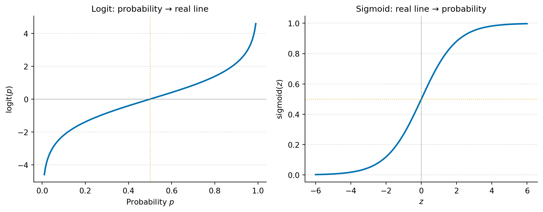
Three properties make logarithms indispensable in practice. First, they turn multiplication into addition: $\ln(ab) = \ln(a) + \ln(b)$. This is why log-likelihoods are easier to work with than raw likelihoods: products of many small probabilities become sums. This matters computationally, too: multiplying thousands of probabilities together underflows to zero in floating-point arithmetic, while summing their logarithms stays numerically stable. Second, they compress dynamic range: $\ln(1{,}000{,}000) \approx 13.8$, so when data spans several orders of magnitude (incomes, populations, word frequencies), a log scale makes patterns visible. Third, they are the basis of the logit transform: $\text{logit}(p) = \ln\!\left(\frac{p}{1-p}\right)$, which maps probabilities in $(0, 1)$ to the entire real line, the foundation of logistic regression.
```{python}
#| label: fig-logit-sigmoid
#| echo: true
#| fig-cap: "The logit function maps probabilities (0, 1) to the full real line; the sigmoid function maps back. Logistic regression works in logit space — where linear relationships are natural — then converts predictions to probabilities via the sigmoid."
#| fig-alt: "Two plots showing inverse functions. The first plot shows the logit function: as probability p increases from 0 to 1 on the x-axis, the output rises steeply towards large negative values near p = 0 and large positive values near p = 1 (the function tends to negative and positive infinity at the limits), crossing zero at p = 0.5. The second plot shows the sigmoid function: as the input z increases from -6 to 6, the output rises from near 0 to near 1, crossing 0.5 at z = 0. Together they illustrate that logit and sigmoid are inverses of each other."
p = np.linspace(0.01, 0.99, 200)
z = np.linspace(-6, 6, 200)

fig, (ax1, ax2) = plt.subplots(1, 2, figsize=(10, 4))
fig.patch.set_alpha(0)

# Left: logit
ax1.patch.set_alpha(0)
ax1.plot(p, np.log(p / (1 - p)), color='#0072B2', linewidth=2)
ax1.axhline(0, color='grey', linewidth=0.8, linestyle='-', alpha=0.5)
ax1.axvline(0.5, color='#E69F00', linewidth=1, linestyle=':', alpha=0.7)
ax1.set_xlabel('Probability $p$')
ax1.set_ylabel('logit($p$)')
ax1.set_title('Logit: probability → real line', fontsize=11)
ax1.spines['top'].set_visible(False)
ax1.spines['right'].set_visible(False)
ax1.yaxis.grid(True, linestyle=':', alpha=0.4, color='grey')
ax1.set_axisbelow(True)

# Right: sigmoid (inverse logit)
ax2.patch.set_alpha(0)
ax2.plot(z, 1 / (1 + np.exp(-z)), color='#0072B2', linewidth=2)
ax2.axhline(0.5, color='#E69F00', linewidth=1, linestyle=':', alpha=0.7)
ax2.axvline(0, color='grey', linewidth=0.8, linestyle='-', alpha=0.5)
ax2.set_xlabel('$z$')
ax2.set_ylabel('sigmoid($z$)')
ax2.set_title('Sigmoid: real line → probability', fontsize=11)
ax2.spines['top'].set_visible(False)
ax2.spines['right'].set_visible(False)
ax2.yaxis.grid(True, linestyle=':', alpha=0.4, color='grey')
ax2.set_axisbelow(True)

plt.tight_layout()
plt.show()
```
## Calculus essentials {#sec-calculus}
Most of the calculus you need for this book reduces to two ideas: derivatives tell you the rate of change, and integrals tell you the area under a curve.
### Derivatives
The **derivative** of a function $f(x)$ at a point tells you how quickly $f$ changes as $x$ changes. In Python terms, it is the slope of the function at that point.
$$
f'(x) = \frac{df}{dx} = \lim_{h \to 0} \frac{f(x+h) - f(x)}{h}
$$
In plain terms: the derivative measures how much the output changes per unit change in input, as that change becomes infinitesimally small. You rarely need to compute derivatives by hand in data science; optimisation libraries and automatic differentiation frameworks (PyTorch, JAX) handle that. But recognising what a derivative *means* is essential, because every model-fitting algorithm is solving "find the parameter values where the derivative of the loss function equals zero."
```{python}
#| label: fig-derivative-example
#| echo: true
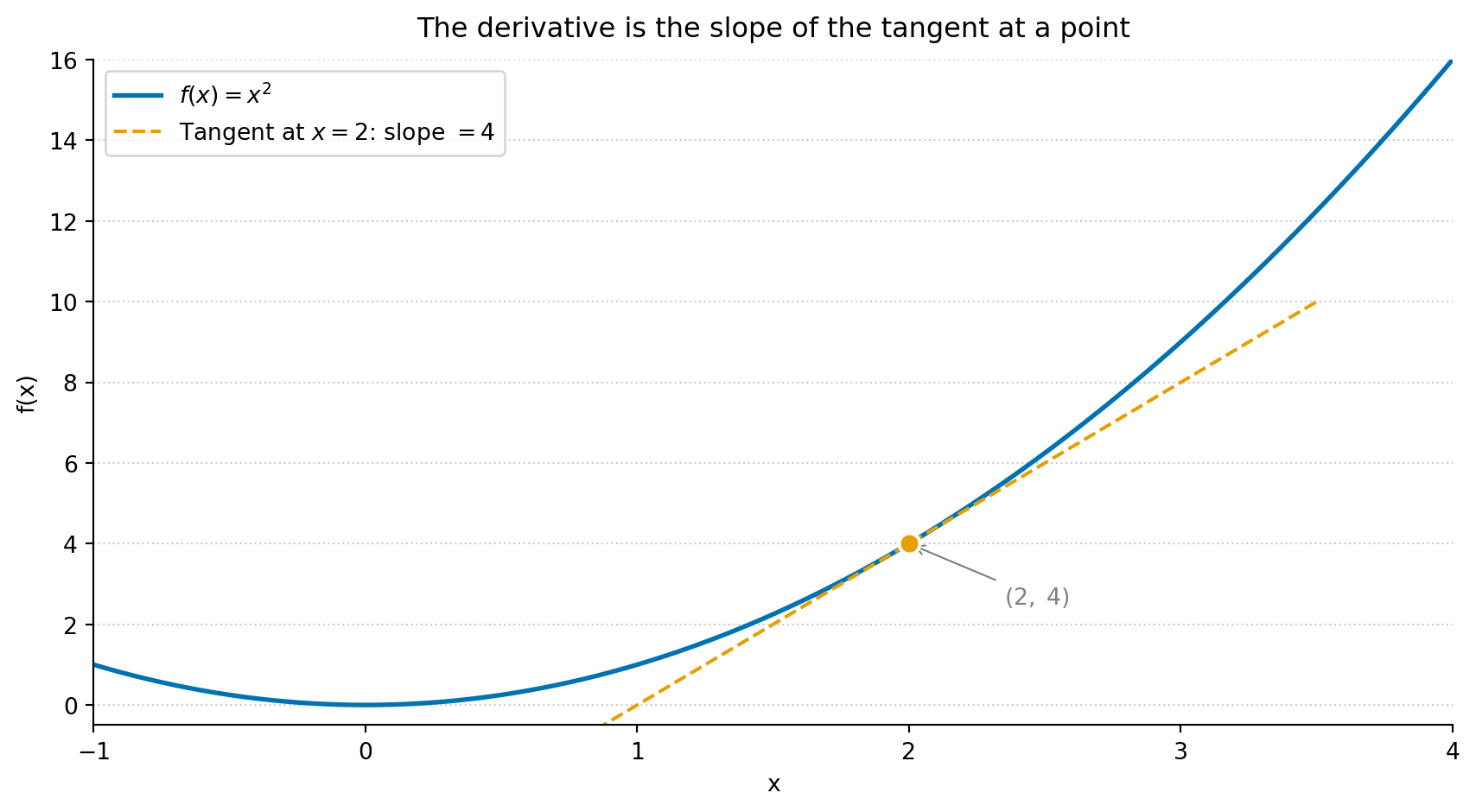
#| fig-cap: "The derivative of f(x) = x² is 2x. At x = 2, the slope is 4 — the tangent line touches the curve and shows the instantaneous rate of change. Gradient descent uses exactly this value to decide which direction to step."
#| fig-alt: "A plot of f(x) = x squared as a solid curve, with a dashed tangent line segment touching the curve at the annotated point (2, 4). A filled circle marks the tangency point. The tangent line's slope of 4 illustrates the derivative at that point."
x = np.linspace(-1, 4, 200)
f = x ** 2

# Tangent line at x0: y = f(x0) + f'(x0)(x - x0)
x0 = 2
f_x0 = x0 ** 2       # f(2) = 4
slope = 2 * x0        # f'(2) = 4

# Clip the tangent to a narrow window around the tangency point
tangent_x = np.linspace(0.5, 3.5, 100)
tangent_y = f_x0 + slope * (tangent_x - x0)

fig, ax = plt.subplots(figsize=(9, 5))
fig.patch.set_alpha(0)
ax.patch.set_alpha(0)
ax.set_title('The derivative is the slope of the tangent at a point',
             fontsize=12, pad=10)
ax.plot(x, f, color='#0072B2', linewidth=2, label=r'$f(x) = x^2$')
ax.plot(tangent_x, tangent_y, color='#E69F00', linewidth=1.5, linestyle='--',
        label=rf"Tangent at $x={x0}$: slope $= {slope}$")
ax.plot(x0, f_x0, 'o', color='#E69F00', markersize=9,
        markeredgecolor='white', markeredgewidth=1.5, zorder=5)
ax.annotate(f'$({x0},\;{f_x0})$', xy=(x0, f_x0),
            xytext=(x0 + 0.35, f_x0 - 1.5), fontsize=10,
            arrowprops=dict(arrowstyle='->', color='grey', lw=0.8),
            color='grey')
ax.set_xlim(-1, 4)
ax.set_ylim(-0.5, 16)
ax.set_xlabel('x')
ax.set_ylabel('f(x)')
ax.legend()
ax.spines['top'].set_visible(False)
ax.spines['right'].set_visible(False)
ax.yaxis.grid(True, linestyle=':', alpha=0.4, color='grey')
ax.set_axisbelow(True)
plt.tight_layout()
plt.show()
```
When a function has multiple inputs, **partial derivatives** measure the rate of change with respect to one variable while holding the others constant. The notation changes from $\frac{d}{dx}$ to $\frac{\partial}{\partial x}$.
The **gradient** $\nabla f$ is the vector of all partial derivatives. It points in the direction of steepest increase. **Gradient descent** — the most common optimisation algorithm in machine learning — works by repeatedly stepping in the opposite direction: downhill towards a minimum.
::: {.callout-tip}
## Author's Note
Every model-fitting algorithm in this book (e.g., least squares regression, logistic regression, gradient-boosted trees) is doing the same thing at its core: searching for parameter values that minimise a loss function. The derivative is the compass that tells the algorithm which direction to step. Once you see that, the zoo of algorithms stops looking like a collection of unrelated methods and starts looking like variations on a single theme: define a loss, take the gradient, step downhill, repeat.
:::
### Integrals
An **integral** computes the area under a curve. For a probability density function (PDF), the area under the curve between two points gives the probability of observing a value in that range.
$$
P(a \leq X \leq b) = \int_a^b f(x)\, dx
$$
The total area under any valid PDF equals 1 (certainty that *some* value will be observed).
```{python}
#| label: fig-integral-example
#| echo: true
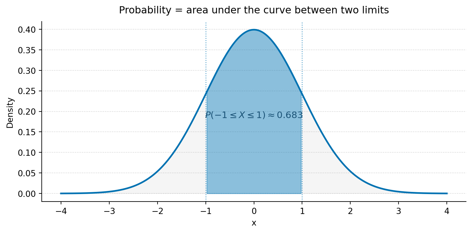
#| fig-cap: "The shaded area under the standard Normal PDF (mean 0, standard deviation 1) between -1 and 1 gives P(-1 ≤ X ≤ 1) ≈ 0.683 — about 68% of the distribution."
#| fig-alt: "A standard Normal bell curve. The central region between x = -1 and x = 1 is shaded, representing approximately 68.3% of the distribution's total area. The tails beyond plus and minus 1 are lightly shaded in grey. Dotted vertical lines mark the integration limits. The probability P(-1 ≤ X ≤ 1) ≈ 0.683 is annotated on the figure."
from scipy import stats

x = np.linspace(-4, 4, 300)
y = stats.norm.pdf(x)

fig, ax = plt.subplots(figsize=(8, 4))
fig.patch.set_alpha(0)
ax.patch.set_alpha(0)
ax.set_title('Probability = area under the curve between two limits',
             fontsize=12, pad=10)
ax.plot(x, y, color='#0072B2', linewidth=2)

# Faint tail shading to show what is excluded
tail_mask = (x < -1) | (x > 1)
ax.fill_between(x, y, where=tail_mask, alpha=0.15, color='grey')

# Shade the area between -1 and 1
mask = (x >= -1) & (x <= 1)
ax.fill_between(x[mask], y[mask], alpha=0.45, color='#0072B2')

# Vertical markers at integration limits
ax.axvline(-1, color='#0072B2', linewidth=1, linestyle=':', alpha=0.7)
ax.axvline( 1, color='#0072B2', linewidth=1, linestyle=':', alpha=0.7)

# Direct annotation instead of distant legend
ax.text(0, 0.18, r'$P(-1 \leq X \leq 1) \approx 0.683$',
        ha='center', va='bottom', fontsize=11, color='#0072B2',
        fontweight='bold')

ax.set_xlabel('x')
ax.set_ylabel('Density')
ax.spines['top'].set_visible(False)
ax.spines['right'].set_visible(False)
ax.yaxis.grid(True, linestyle=':', alpha=0.4, color='grey')
ax.set_axisbelow(True)
plt.tight_layout()
plt.show()
```
In practice, you will rarely compute integrals yourself. The `scipy.stats` CDF method does it for you: `stats.norm.cdf(1) - stats.norm.cdf(-1)` gives the same 0.683 as the shaded area above.
## Linear algebra essentials {#sec-linear-algebra}
Linear algebra provides the language for working with collections of numbers simultaneously. In data science, your data almost always lives in a matrix (rows = observations, columns = features), and you express most algorithms as matrix operations.
### Vectors
A **vector** is an ordered list of numbers. In Python, it is a one-dimensional NumPy array.
$$
\mathbf{x} = \begin{bmatrix} x_1 \\ x_2 \\ x_3 \end{bmatrix}
$$
The **dot product** of two vectors multiplies corresponding elements and sums the results:
$$
\mathbf{x} \cdot \mathbf{y} = \sum_{i=1}^{n} x_i y_i
$$
This is the core operation behind linear regression: a predicted value is the dot product of features and coefficients.
```{python}
#| label: dot-product-example
#| echo: true
x = np.array([2, 3, 5])
y = np.array([1, 4, 2])

# These are all equivalent
print(f"np.dot:        {np.dot(x, y)}")
print(f"@ operator:    {x @ y}")
print(f"Manual sum:    {sum(a * b for a, b in zip(x, y))}")
```
### Matrices
A **matrix** is a two-dimensional array of numbers. In data science, your feature matrix $\mathbf{X}$ typically has $n$ rows (observations) and $p$ columns (features).
$$
\mathbf{X} = \begin{bmatrix}
x_{11} & x_{12} \\
x_{21} & x_{22} \\
x_{31} & x_{32}
\end{bmatrix}
$$
The **transpose** $\mathbf{X}^T$ swaps rows and columns. **Matrix multiplication** $\mathbf{A}\mathbf{B}$ requires the number of columns of $\mathbf{A}$ to equal the number of rows of $\mathbf{B}$; the inner dimensions must match. In NumPy, the `@` operator handles both dot products and matrix multiplication.
```{python}
#| label: matrix-example
#| echo: true
X = np.array([[1, 2],
              [3, 4],
              [5, 6]])

print(f"X shape:    {X.shape}")      # (3, 2)
print(f"X^T shape:  {X.T.shape}")    # (2, 3)

# X^T @ X gives a (2, 2) matrix — this appears in the
# normal equations for linear regression
print(f"\nX^T @ X:\n{X.T @ X}")
```
::: {.callout-note}
## Engineering Bridge
Matrix multiplication is how ML frameworks batch-process multiple observations simultaneously. When you see `X @ w` in a model's forward pass, that is $n$ simultaneous dot products — one per row of $\mathbf{X}$. The `@` operator in NumPy maps directly to optimised BLAS routines, which is why vectorised matrix operations are orders of magnitude faster than Python `for` loops over individual rows. If you have ever profiled a hot loop and replaced it with a single library call, the same instinct applies here.
:::
### Matrix inversion {#sec-matrix-inversion}
The **inverse** of a square matrix $\mathbf{A}$, written $\mathbf{A}^{-1}$, is the matrix that satisfies $\mathbf{A}\mathbf{A}^{-1} = \mathbf{I}$, where $\mathbf{I}$ is the identity matrix. Think of it as the matrix equivalent of division: dividing by $5$ means multiplying by $5^{-1}$, and inverting a matrix plays the same role. Not every matrix has an inverse — those that don't are called **singular**, and they are the matrix analogue of dividing by zero. The closed-form OLS solution you fit in @sec-statsmodels-ols,
$$
\hat{\boldsymbol{\beta}} = (\mathbf{X}^T \mathbf{X})^{-1} \mathbf{X}^T \mathbf{y},
$$
contains exactly one such inversion. `np.linalg.inv(X.T @ X)` will compute it for you, but this is rarely how production libraries solve the normal equations, for the reason below.
A matrix can be technically invertible but still **ill-conditioned**: close enough to singular that floating-point arithmetic gives you coefficients that are exquisitely sensitive to tiny changes in the input. The **condition number** is the standard diagnostic — the ratio of the largest to the smallest singular value — and `np.linalg.cond(X)` returns it. Large values signal trouble: two predictors that are nearly collinear, or features on wildly different scales (the warning you meet in Chapter 9 at @sec-multiple-regression is this), can push the condition number into the thousands or more. `statsmodels` doesn't actually invert $\mathbf{X}^T \mathbf{X}$ directly; it solves the same linear system via QR or pinv decompositions, which preserve more accuracy when the matrix is badly conditioned. If you ever need to compute $(\mathbf{X}^T\mathbf{X})^{-1}$ for inference (to get coefficient variances, say), prefer `np.linalg.pinv` or `scipy.linalg.solve` over `np.linalg.inv` for the same reason.
```{python}
#| label: matrix-inversion-example
#| echo: true
# A well-conditioned 2x2 system
A = np.array([[4.0, 1.0],
              [2.0, 3.0]])
A_inv = np.linalg.inv(A)

print(f"A @ A_inv:\n{A @ A_inv}")      # approximately the identity
print(f"\ncond(A) = {np.linalg.cond(A):.2f}")   # small → well-behaved

# A nearly-collinear feature matrix: condition number blows up
X_bad = np.array([[1.0, 1.0],
                  [1.0, 1.0001],
                  [1.0, 0.9999]])
print(f"\ncond(X^T X) = {np.linalg.cond(X_bad.T @ X_bad):.2e}")
```
### Eigenvalues and eigenvectors
If you have a system described by several correlated metrics — CPU usage, memory consumption, request latency — the metrics tend to move together. **Eigenvectors** of the covariance matrix identify the independent "directions of variation" in that system: the distinct ways the metrics co-move as a unit. **Eigenvalues** measure how much variation each direction captures.
Formally, an eigenvector of a matrix $\mathbf{A}$ is a vector whose direction doesn't change when $\mathbf{A}$ is applied to it (up to a sign flip if the eigenvalue is negative). It only gets scaled by a factor, the eigenvalue (conventionally written $\lambda$ in this context, distinct from the rate parameter $\lambda$ in @tbl-greek-letters); for a covariance matrix, which is positive semi-definite, the eigenvalues are non-negative, so the direction is genuinely preserved:
$$
\mathbf{A}\mathbf{v} = \lambda\mathbf{v}
$$
This concept is central to dimensionality reduction (PCA): the eigenvectors of the covariance matrix define the principal component directions, and the eigenvalues tell you how much variance each component captures.
```{python}
#| label: eigen-example
#| echo: true
# Covariance matrix of two correlated features
C = np.array([[2.0, 1.2],
              [1.2, 1.0]])

eigenvalues, eigenvectors = np.linalg.eigh(C)

# eigh returns ascending order; reverse to match PCA convention (largest first)
idx = np.argsort(eigenvalues)[::-1]
eigenvalues = eigenvalues[idx]
eigenvectors = eigenvectors[:, idx]

print('Eigenvalues:', eigenvalues)
print('Eigenvectors (columns):')
print(eigenvectors)
pct = eigenvalues / eigenvalues.sum() * 100
print(f"\nVariance explained: PC1={pct[0]:.1f}%, PC2={pct[1]:.1f}%")
```
The first component captures about 93% of the variance: in PCA terms, you could represent this two-dimensional data with a single number and lose very little information.
## Probability notation {#sec-probability-notation}
Probability has its own compact notation. Here is the vocabulary you need.
| Notation | Read as | Meaning |
| :--------: | :------- | :------- |
| $P(A)$ | "probability of A" | How likely event $A$ is (between 0 and 1) |
| $P(A \mid B)$ | "probability of A given B" | How likely $A$ is, knowing $B$ occurred |
| $P(A \cap B)$ | "probability of A and B" | Both $A$ and $B$ occur |
| $P(A \cup B)$ | "probability of A or B" | At least one of $A$ or $B$ occurs |
| $X \sim N(\mu, \sigma^2)$ | "X follows a Normal" | $X$ is drawn from a Normal with mean $\mu$ and variance $\sigma^2$ |
| $E[X]$ | "expected value of X" | The long-run average; $E[X] = \mu$ |
| $\text{Var}(X)$ | "variance of X" | The expected squared deviation from the mean |
: Probability notation reference. {#tbl-probability-notation}
A note on the Normal distribution parameterisation: the mathematical convention $N(\mu, \sigma^2)$ uses the *variance* as the second parameter. In `scipy`, however, `stats.norm(loc=mu, scale=sigma)` takes the *standard deviation*. Both refer to the same distribution; just be aware which parameterisation a given source is using.
The core rules that connect these symbols are:
Complement rule
: $P(\text{not } A) = 1 - P(A)$
Addition rule
: $P(A \cup B) = P(A) + P(B) - P(A \cap B)$
Multiplication rule
: $P(A \cap B) = P(A) \times P(B \mid A)$
Bayes' theorem
: $P(A \mid B) = \dfrac{P(B \mid A) \times P(A)}{P(B)}$
Bayes' theorem is the engine behind an entire branch of statistics. It tells you how to update a belief: start with what you believed before observing data — the **prior**, $P(A)$. Measure how well your hypothesis predicts what you observed — the **likelihood**, $P(B \mid A)$. Normalise by the overall probability of the observation — the **evidence**, $P(B)$. The result is your updated belief — the **posterior**, $P(A \mid B)$.
```{python}
#| label: bayes-example
#| echo: true
# A medical screening test:
#   - 1% of the population has the condition (prior)
#   - The test correctly detects 95% of true cases (sensitivity)
#   - The test incorrectly flags 5% of healthy people (false positive rate)

p_condition = 0.01                     # P(condition)
p_positive_given_condition = 0.95      # P(positive | condition)
p_positive_given_healthy = 0.05        # P(positive | no condition)

# Law of total probability for the denominator
p_positive = (p_positive_given_condition * p_condition
              + p_positive_given_healthy * (1 - p_condition))

# Bayes: posterior
p_condition_given_positive = (p_positive_given_condition * p_condition) / p_positive
print(f"P(condition | positive test) = {p_condition_given_positive:.3f}")
print(f"Despite a 95%-sensitive test, a positive result means only a"
      f" {p_condition_given_positive:.0%} chance of having the condition.")
```
## Distribution notation {#sec-distribution-notation}
A **probability distribution** describes the possible values of a random variable and how likely each one is. The notation differs slightly between discrete and continuous distributions.
For **discrete** distributions (outcomes you can count), the **probability mass function** (PMF) gives the probability of each specific outcome:
$$
P(X = k) \quad \text{e.g., } P(X = 3) = 0.18
$$
For **continuous** distributions (outcomes on a smooth scale), the **probability density function** (PDF) gives the *density* at each point. Probabilities come from integrating the PDF over an interval; the density at a single point is not itself a probability.
Both types share a **cumulative distribution function** (CDF):
$$
F(x) = P(X \leq x)
$$
Both types also have an inverse CDF, the **quantile function** (called `ppf` in `scipy`), which answers "what value has $q$% of the distribution below it?"
```{python}
#| label: distribution-notation-example
#| echo: true
# Discrete: Poisson(λ=5)
poisson = stats.poisson(mu=5)
print(f"PMF: P(X = 3) = {poisson.pmf(3):.4f}")
print(f"CDF: P(X ≤ 3) = {poisson.cdf(3):.4f}")
print(f"PPF: value at 95th percentile = {poisson.ppf(0.95):.0f}")

# Continuous: Normal(μ=0, σ²=1)
normal = stats.norm(loc=0, scale=1)  # scale is σ (standard deviation)
print(f"\nPDF: f(0)     = {normal.pdf(0):.4f}")
print(f"CDF: P(X ≤ 0) = {normal.cdf(0):.4f}")
print(f"PPF: value at 97.5th percentile = {normal.ppf(0.975):.4f}")
```
## Common formulae {#sec-common-formulae}
These formulae recur throughout the book. Each is paired with its NumPy equivalent.
**Sample mean:**
$$
\bar{x} = \frac{1}{n}\sum_{i=1}^{n} x_i
$$
**Sample variance** (with Bessel's correction, dividing by $n - 1$ rather than $n$ to correct for the slight downward bias when estimating population variance from a sample):
$$
s^2 = \frac{1}{n-1}\sum_{i=1}^{n}(x_i - \bar{x})^2
$$
**Standard deviation** is the square root of variance: $s = \sqrt{s^2}$.
**Standard error of the mean** measures how precisely you've estimated the population mean:
$$
\text{SE} = \frac{s}{\sqrt{n}}
$$
```{python}
#| label: common-formulas
#| echo: true
x = np.array([12, 15, 14, 10, 13, 16, 11, 14, 15, 12])

# Mean
mean = np.mean(x)
print(f"Mean: {mean}")

# Variance (ddof=1 for sample variance — Bessel's correction)
variance = np.var(x, ddof=1)
print(f"Variance: {variance:.2f}")

# Standard deviation
std = np.std(x, ddof=1)
print(f"Standard deviation: {std:.2f}")

# Standard error of the mean
se = std / np.sqrt(len(x))
print(f"Standard error: {se:.2f}")
```
Notice the $\sqrt{n}$ in the denominator of the standard error: quadrupling your sample size halves your standard error. This square-root relationship between data volume and precision is one of the most important practical facts in statistics, and it explains the diminishing returns of simply collecting more data. To halve your standard error you must quadruple your sample size, so each further halving costs four times the data as the one before. If a single observation gives $\text{SE} = 1$, then going from 100 to 400 observations buys a reduction in SE from $0.1$ to $0.05$, but the next halving demands 1,600 observations, the one after that 6,400, and so on. Every quadrupling still halves the SE; it is the absolute gain that shrinks, because you are halving an already-small number while paying ever more for the privilege.
## Set notation {#sec-set-notation}
Sets appear in probability contexts. The notation maps directly to concepts you know from programming.
| Symbol | Meaning | Python equivalent |
| :------: | :------- | :----------------- |
| $\in$ | "is a member of" | `x in S` |
| $\cup$ | Union (or) | <code>A | B</code> (sets) |
| $\cap$ | Intersection (and) | `A & B` (sets) |
| $\subseteq$ | Subset (possibly equal) | `A <= B` or `A.issubset(B)` |
| $\subset$ | Proper subset ($A \neq B$) | `A < B` |
| $\emptyset$ | Empty set | `set()` |
| $\mathbb{R}$ | All real numbers | `float` (conceptually) |
| $\mathbb{R}^n$ | $n$-dimensional real space | `np.ndarray` of shape `(n,)` |
: Set notation and Python equivalents. {#tbl-set-notation}