---
# Content: CC BY-NC-SA 4.0 | Code: MIT - see /LICENSE.md
title: "Building a recommendation system"
---
{{< include /_common-imports.qmd >}}
## The problem every platform has {#sec-recsys-intro}
You've built search. Users type a query, your system returns results ranked by relevance, and the interaction ends. But what happens when the user opens your app and doesn't type anything? The blank landing page is the hardest screen in product engineering: you need to show something useful before the user tells you what they want. Every time Netflix surfaces a row of films, Spotify generates a playlist, or an e-commerce site shows "customers also bought," a recommendation system is making predictions about human preferences from incomplete data.
This is a different kind of prediction from what we've seen so far. Churn prediction (@sec-churn-intro) asked a binary question — will this customer leave? Regression (@sec-from-description-to-prediction) predicted a continuous value. Recommendation systems predict a *matrix* of preferences (every user's opinion of every item) from a dataset where the vast majority of entries are missing. A platform with 100,000 users and 10,000 items has a billion possible user-item pairs, but a typical user interacts with only a few dozen items, so well over 99% of the matrix is empty.
The engineering challenge is familiar: you're building a system that must serve personalised results at low latency for millions of users. The data science challenge is less familiar: you're estimating preferences from sparse, noisy, implicit signals, and the thing you're predicting (human taste) is subjective, context-dependent, and constantly shifting.
## The interaction matrix {#sec-interaction-matrix}
The foundation of most recommendation systems is the **interaction matrix** (also called the user-item matrix or ratings matrix). Each row is a user, each column is an item, and each entry records an interaction: a rating, a purchase, a click, or simply whether the user engaged with the item at all.
```{python}
#| label: interaction-matrix-setup
#| echo: true
rng = np.random.default_rng(42)

n_users = 500
n_items = 200
n_interactions = 15000  # ~15% density — sparse, though denser than production

# Simulate user and item latent factors (hidden preferences and attributes)
n_factors = 3
user_factors = rng.normal(0, 1, (n_users, n_factors))
item_factors = rng.normal(0, 1, (n_items, n_factors))

# True preferences are the dot products of the latent factors, standardised
# to unit scale so we can map them onto the 1–5 rating range predictably.
true_preferences = user_factors @ item_factors.T
true_preferences /= true_preferences.std()

# Sample which user-item pairs are observed (not random — biased towards
# items the user would prefer, mimicking real browsing behaviour). The
# temperature softens that bias: without it, users would only ever see their
# handful of top favourites, and every observed rating would be a 5.
observed_pairs = set()
temperature = 2.2
while len(observed_pairs) < n_interactions:
    u = rng.integers(0, n_users)
    weights = np.exp(true_preferences[u] / temperature)
    weights /= weights.sum()
    i = rng.choice(n_items, p=weights)
    observed_pairs.add((u, i))

# Generate ratings (1–5) from true preferences plus noise. The intercept and
# scale are chosen so ratings span the whole scale rather than piling up at 5.
rows = []
for u, i in observed_pairs:
    rating = np.clip(
        np.round(3.2 + 1.5 * true_preferences[u, i] + rng.normal(0, 0.3)), 1, 5
    )
    rows.append({'user_id': u, 'item_id': i, 'rating': int(rating)})

ratings_df = pd.DataFrame(rows)
print(f"Users: {n_users:,}")
print(f"Items: {n_items:,}")
print(f"Interactions: {len(ratings_df):,}")
print(f"Matrix density: {len(ratings_df) / (n_users * n_items):.1%}")
print(f"Rating distribution:")
print(ratings_df['rating'].value_counts().sort_index().to_string())
```
The 15% density we've simulated is generous; real-world systems often have densities below 1%. This sparsity is the central technical challenge. Most machine learning algorithms assume you have complete feature vectors for each observation. Here, the "feature vector" is the user's preference for every item, and almost all of it is missing.
::: {.callout-note}
## Engineering Bridge
The interaction matrix is the adjacency matrix of a **bipartite graph**: users and items are two distinct node types, and edges only run between them (users rate items, never other users). The matrix is rectangular, not square, which distinguishes it from the symmetric adjacency matrices in general graph problems. But the storage patterns are identical: you wouldn't materialise a billion-cell dense matrix when only a fraction of edges exist. Recommendation systems work with sparse representations: coordinate lists, compressed sparse row (CSR) formats, or simply DataFrames of (user, item, value) triples. If you've worked with sparse data structures in graph processing or network analysis, the indexing and traversal patterns will be familiar.
:::
## Collaborative filtering: users who liked this also liked that {#sec-collaborative-filtering}
**Collaborative filtering** is the idea that users who agreed in the past will agree in the future. If you and I both rated the same ten films highly, and you loved a film I haven't seen, there's a reasonable chance I'd like it too. The algorithm doesn't need to know *anything* about what the films are; it works entirely from the pattern of interactions.
There are two flavours. **User-based** collaborative filtering finds users similar to you and recommends items they liked. **Item-based** collaborative filtering finds items similar to ones you've liked and recommends those. The mechanics are nearly identical; they differ only in which axis of the interaction matrix you compute similarity over.
Let's implement item-based collaborative filtering. For each pair of items, we compute the **cosine similarity** between their columns in the interaction matrix, treating each item as a vector of user ratings. Items that receive similar ratings from the same users will have high similarity.
```{python}
#| label: item-based-cf
#| echo: true
from scipy.sparse import csr_matrix
from sklearn.metrics.pairwise import cosine_similarity

# Build sparse interaction matrix
interaction_matrix = csr_matrix(
    (ratings_df['rating'].values,
     (ratings_df['user_id'].values, ratings_df['item_id'].values)),
    shape=(n_users, n_items)
)

# Compute item-item similarity (cosine similarity between item columns)
item_similarity = cosine_similarity(interaction_matrix.T)
np.fill_diagonal(item_similarity, 0)  # don't recommend an item to itself

def recommend_items_cf(user_id, interaction_matrix, item_similarity, n=5):
    """Recommend items using item-based collaborative filtering."""
    user_ratings = interaction_matrix[user_id].toarray().flatten()
    rated_mask = user_ratings > 0

    # Predicted score: similarity-weighted average of the user's known ratings
    scores = item_similarity @ user_ratings
    # Normalise by the sum of absolute similarities to rated items
    sim_sums = np.abs(item_similarity[:, rated_mask]).sum(axis=1)
    sim_sums[sim_sums == 0] = 1  # avoid division by zero
    scores = scores / sim_sums

    # Exclude already-rated items
    scores[rated_mask] = -np.inf
    top_items = np.argsort(scores)[::-1][:n]
    return top_items, scores[top_items]

# Example: recommendations for user 0
rec_items, rec_scores = recommend_items_cf(0, interaction_matrix, item_similarity)
user_history = ratings_df[ratings_df['user_id'] == 0].sort_values('rating', ascending=False)

print(f"User 0 has rated {len(user_history)} items")
print(f"Top-rated items: {user_history.head(3)[['item_id', 'rating']].to_string(index=False)}")
print(f"\nRecommended items: {rec_items}")
print(f"Predicted scores:  {np.round(rec_scores, 2)}")
```
The approach is intuitive and requires no training: you compute similarities once and generate recommendations on the fly. But it has significant limitations. Similarity computation is $O(n^2)$ in the number of items (or users), which doesn't scale well. More fundamentally, it can only recommend items that share rating patterns with items you've already rated; it struggles with the **long tail** of items that have few ratings.
## Matrix factorisation: compressing preferences {#sec-matrix-factorisation}
Matrix factorisation takes a different approach. Instead of computing pairwise similarities, it decomposes the interaction matrix into two smaller matrices, one representing users and one representing items, in a shared low-dimensional latent space. If PCA (@sec-pca) finds the directions of maximum variance in a feature matrix, matrix factorisation finds the latent dimensions that best explain the observed ratings.
The idea is that a user's rating of an item can be approximated as the dot product of a user vector and an item vector:
$$
\hat{r}_{ui} = \mathbf{p}_u \cdot \mathbf{q}_i = \sum_{k=1}^{K} p_{uk} \, q_{ik}
$$
where $\mathbf{p}_u$ is a $K$-dimensional vector representing user $u$'s preferences, $\mathbf{q}_i$ is a $K$-dimensional vector representing item $i$'s attributes, and $K$ is the number of latent factors (typically 10–100 — not to be confused with $K$ for the number of classes in @sec-multiclass or clusters in @sec-kmeans). Each factor might correspond to something interpretable: one dimension might capture "action versus drama," another "mainstream versus indie." But the algorithm discovers these dimensions automatically from the data. This is the same principle behind the latent components in PCA and the latent topics in text analysis: compress high-dimensional data by finding its underlying structure.
We find $\mathbf{P}$ and $\mathbf{Q}$ by minimising the reconstruction error on observed ratings, with regularisation to prevent overfitting:
$$
\min_{\mathbf{P}, \mathbf{Q}} \sum_{(u, i) \in \text{observed}} \left( r_{ui} - \mathbf{p}_u \cdot \mathbf{q}_i \right)^2 + \alpha \sum_u \|\mathbf{p}_u\|^2 + \alpha \sum_i \|\mathbf{q}_i\|^2
$$
In words: minimise the squared error on observed ratings, plus an L2 penalty on every user and item vector. The regularisation term $\alpha$ plays exactly the same role as in ridge regression (@sec-ridge): it penalises large parameter values to keep the model from fitting noise in the sparse observed data. A common extension adds explicit bias terms: a global mean $\mu$, a per-user bias $b_u$ (some users rate everything higher), and a per-item bias $b_i$ (some items are systematically better-received), so the prediction becomes $\hat{r}_{ui} = \mu + b_u + b_i + \mathbf{p}_u \cdot \mathbf{q}_i$. Our simplified formulation omits these for clarity, but in production they often capture a large fraction of the variance.
```{python}
#| label: matrix-factorisation
#| echo: true
from sklearn.decomposition import TruncatedSVD

# For demonstration, we'll use truncated SVD. SVD treats missing entries as
# zeros — implicitly telling the model that every unrated item has a rating of
# 0, far below the 1–5 observed scale, which systematically depresses the
# reconstructions. We mitigate this the standard way: subtract the global mean
# rating before factorising, so a missing (zero) entry now represents an
# *average* rating rather than a terrible one, then add the mean back when
# reconstructing. In production you'd go further, using alternating least
# squares (ALS) or stochastic gradient descent (SGD) that optimise only over
# observed entries. SVD is illustrative and ships with scikit-learn.
global_mean = ratings_df['rating'].mean()

# Centre only the observed entries; unobserved entries stay 0, now meaning "mean".
centred_matrix = csr_matrix(
    (ratings_df['rating'].values - global_mean,
     (ratings_df['user_id'].values, ratings_df['item_id'].values)),
    shape=(n_users, n_items)
)

n_components = 20
svd = TruncatedSVD(n_components=n_components, random_state=42)

# fit_transform returns U @ Sigma — singular values are already absorbed
user_latent = svd.fit_transform(centred_matrix)      # (n_users, n_components)
# components_ is V^T, so .T gives V
item_latent = svd.components_.T                       # (n_items, n_components)

print(f"User latent matrix: {user_latent.shape}")
print(f"Item latent matrix: {item_latent.shape}")
print(f"Explained variance ratio: {svd.explained_variance_ratio_.sum():.1%}")

# Reconstruct ratings for user 0: (U @ Sigma) @ V^T, plus the global mean
reconstructed_ratings = user_latent[0] @ item_latent.T + global_mean
actual_ratings = interaction_matrix[0].toarray().flatten()
rated_items = np.where(actual_ratings > 0)[0]

comparison = pd.DataFrame({
    'item_id': rated_items,
    'actual': actual_ratings[rated_items],
    'reconstructed': np.round(reconstructed_ratings[rated_items], 1)
}).head(10)
print(f"\nUser 0 — actual vs reconstructed ratings (in-sample):")
print(comparison.to_string(index=False))
```
This is an *in-sample reconstruction*, not a prediction. The SVD was fitted on the full interaction matrix, so it has already seen user 0's ratings; comparing reconstructed against actual values here only checks that the factorisation has captured real structure, and it will always flatter the model because nothing has been held out. We measure honest performance on held-out interactions later, in @sec-recsys-evaluation.
```{python}
#| label: fig-latent-space
#| echo: true
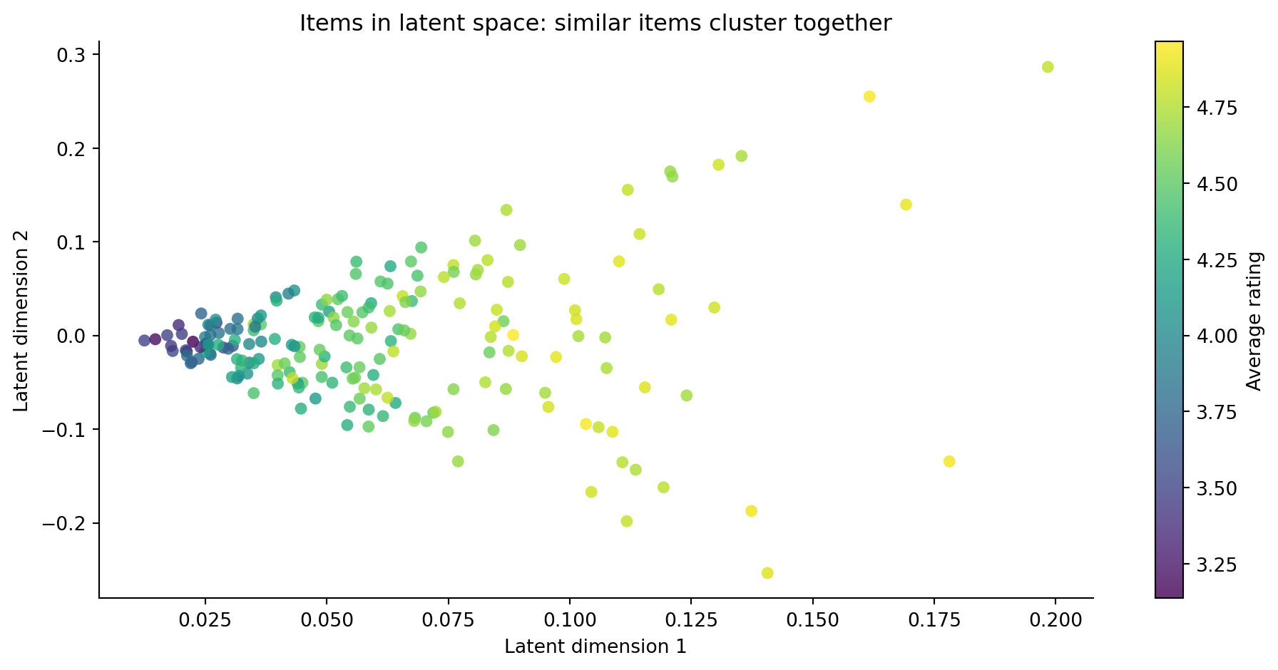
#| fig-cap: "Items projected into a two-dimensional latent space from the matrix factorisation. Clusters of nearby items share similar rating patterns — users who like one item in a cluster tend to like others nearby. Position, not colour, carries the chapter's point; colour shows average rating and marker size shows the number of ratings."
#| fig-alt: "Scatter plot showing 200 items projected onto two latent dimensions from the matrix factorisation. Points are coloured on the viridis sequential scale from dark purple (low average rating) to bright yellow (high average rating), with a colour bar on the right labelled 'Average rating'. Marker size redundantly encodes the number of ratings each item received, so larger points are more-rated items; this channel survives loss of colour. Items with similar rating patterns cluster together in the latent space, demonstrating that the factorisation has learned meaningful preference structure. The key message — similar items cluster — depends on position, not colour."
# Compute average rating per item, excluding unrated entries (zeros).
# .filled(np.nan) makes any unrated item explicitly NaN rather than 0, so it
# renders as a distinct "bad value" colour instead of silently darkest.
# At this scale every item happens to be rated, but the code stays robust.
dense = interaction_matrix.toarray()
masked = np.ma.masked_equal(dense, 0)
avg_ratings = masked.mean(axis=0).filled(np.nan)
n_ratings_per_item = (dense > 0).sum(axis=0)

# Use the first two latent dimensions for visualisation
fig, ax = plt.subplots(figsize=(10, 5))
fig.patch.set_alpha(0)
ax.patch.set_alpha(0)
# Marker size encodes the number of ratings, a redundant channel that
# survives loss of colour (greyscale or low-vision viewing).
sc = ax.scatter(
    item_latent[:, 0], item_latent[:, 1],
    c=avg_ratings,
    s=20 + 4 * n_ratings_per_item,
    cmap='viridis', alpha=0.8, edgecolors='none'
)
cbar = plt.colorbar(sc, ax=ax)
cbar.set_label('Average rating')
ax.set_xlabel('Latent dimension 1')
ax.set_ylabel('Latent dimension 2')
ax.set_title('Items in latent space: similar items cluster together')
ax.spines[['top', 'right']].set_visible(False)
plt.tight_layout()
plt.show()
```
The latent space gives us something collaborative filtering alone doesn't: a compact representation of *why* users and items are similar. Two items close in latent space share underlying attributes that drive similar ratings, even if few users have rated both. This is how matrix factorisation addresses sparsity: it generalises across the gaps by learning structure rather than relying on direct co-occurrence.
::: {.callout-tip}
## Author's Note
Matrix factorisation clicked for me when I stopped thinking of it as a prediction algorithm and started thinking of it as compression. In our simulation, the interaction matrix has 100,000 cells (500 users × 200 items) but only 15,000 are filled in. Yet 20 latent dimensions can reconstruct those 15,000 entries reasonably well — once we centre the ratings to sidestep the zero-imputation trap — which means the underlying structure of human preferences is far lower-dimensional than the raw matrix suggests. It's the same insight behind dimensionality reduction in @sec-pca, but applied to a matrix that's mostly empty. The compression *is* the model: by forcing the data through a bottleneck, you learn what matters and discard what's noise.
:::
## Content-based filtering: using item features {#sec-content-based}
Collaborative filtering works entirely from interaction patterns; it doesn't need to know what items *are*. **Content-based filtering** takes the opposite approach: it recommends items similar to what the user has liked, based on item attributes.
If a user rated several Python programming books highly, a content-based system would recommend other Python books. It examines item features (genre, author, price range, description keywords) and builds a profile of each user's preferences over those features.
```{python}
#| label: content-based
#| echo: true
# Simulate item features: genre, price range, and quality indicators
n_genres = 8
item_genre_probs = rng.dirichlet(np.ones(n_genres) * 0.5, n_items)
item_price = rng.uniform(5, 100, n_items)
item_popularity = rng.exponential(1, n_items)

# Feature matrix: genre distribution + normalised price + popularity
item_content = np.column_stack([
    item_genre_probs,
    (item_price - item_price.mean()) / item_price.std(),
    (item_popularity - item_popularity.mean()) / item_popularity.std(),
])

def recommend_content_based(user_id, interaction_matrix, item_content, n=5):
    """Build a user profile from rated items and find similar unrated items."""
    user_ratings = interaction_matrix[user_id].toarray().flatten()
    rated_mask = user_ratings > 0

    if rated_mask.sum() == 0:
        return np.array([]), np.array([])

    # User profile: weighted average of item features, weighted by rating
    weights = user_ratings[rated_mask]
    user_profile = (item_content[rated_mask].T @ weights) / weights.sum()

    # Score unrated items by cosine similarity to user profile
    scores = cosine_similarity(user_profile.reshape(1, -1), item_content).flatten()
    scores[rated_mask] = -np.inf

    top_items = np.argsort(scores)[::-1][:n]
    return top_items, scores[top_items]

rec_items_cb, rec_scores_cb = recommend_content_based(
    0, interaction_matrix, item_content
)
print(f"Content-based recommendations for user 0: {rec_items_cb}")
print(f"Similarity scores: {np.round(rec_scores_cb, 3)}")
```
The scores reflect how closely each recommended item's features match the user's profile. Notice that content-based scores are bounded between -1 and 1 (cosine similarity), unlike the unbounded predicted ratings from collaborative filtering; the two approaches operate on different scales, which is why the hybrid system below normalises both before combining them.
Content-based filtering has a distinct advantage: it can recommend items with no interaction history at all, as long as you have their features. A new book added to the catalogue can be recommended immediately based on its genre and description — no ratings required. We'll see in @sec-cold-start why this matters so much.
But content-based filtering has its own limitation: it can only recommend items similar to what the user has already seen. It doesn't discover surprising connections: the fact that fans of obscure jazz also tend to enjoy nature documentaries, for instance. Collaborative filtering captures these cross-category patterns because it works from behaviour, not metadata.
## Hybrid systems: combining signals {#sec-hybrid}
Before building a hybrid, it helps to see where each approach excels and where it falls short:
| | Collaborative filtering | Content-based filtering |
| --: | :-- | :-- |
| **Data needed** | User-item interactions | Item features (metadata) |
| **New items** | Cannot recommend (no interactions) | Can recommend immediately |
| **New users** | Cannot personalise (no history) | Cannot personalise (no history) |
| **Cross-category discovery** | Strong — finds surprising patterns | Weak — only recommends similar items |
| **Scalability** | $O(n^2)$ similarity; $O(K)$ with matrix factorisation | $O(\text{items} \times \text{features})$ |
: Comparison of collaborative filtering and content-based filtering across key dimensions. {#tbl-cf-cb-comparison}
In practice, production recommendation systems combine multiple approaches. A **hybrid system** uses collaborative filtering as its primary signal, content-based features to handle cold-start items, and popularity as a fallback for completely new users.
```{python}
#| label: hybrid-recommender
#| echo: true
def recommend_hybrid(user_id, interaction_matrix, item_similarity,
                     item_content, w=0.6, n=5):
    """
    Combine collaborative and content-based scores.

    w controls the weight: 1.0 = pure collaborative, 0.0 = pure content.
    """
    user_ratings = interaction_matrix[user_id].toarray().flatten()
    rated_mask = user_ratings > 0

    # Collaborative filtering scores
    cf_scores = item_similarity @ user_ratings
    sim_sums = np.abs(item_similarity[:, rated_mask]).sum(axis=1)
    sim_sums[sim_sums == 0] = 1
    cf_scores = cf_scores / sim_sums

    # Content-based scores
    if rated_mask.sum() > 0:
        weights = user_ratings[rated_mask]
        user_profile = (item_content[rated_mask].T @ weights) / weights.sum()
        cb_scores = cosine_similarity(
            user_profile.reshape(1, -1), item_content
        ).flatten()
    else:
        cb_scores = np.zeros(n_items)

    # Normalise both to [0, 1] for fair combination
    def min_max_scale(x):
        finite = x[np.isfinite(x)]
        if finite.max() == finite.min():
            return np.zeros_like(x)
        return (x - finite.min()) / (finite.max() - finite.min())

    cf_norm = min_max_scale(cf_scores)
    cb_norm = min_max_scale(cb_scores)

    combined = w * cf_norm + (1 - w) * cb_norm
    combined[rated_mask] = -np.inf

    top_items = np.argsort(combined)[::-1][:n]
    return top_items, combined[top_items]

rec_hybrid, scores_hybrid = recommend_hybrid(
    0, interaction_matrix, item_similarity, item_content
)
print(f"Hybrid recommendations for user 0: {rec_hybrid}")
print(f"Combined scores: {np.round(scores_hybrid, 3)}")
```
The mixing weight $w$ (the `w` parameter in the code) is a hyperparameter you'd tune empirically, and it might vary per user. A user with hundreds of ratings provides strong collaborative signal; a new user with three ratings benefits more from content-based features.
::: {.callout-note}
## Engineering Bridge
A hybrid recommendation system follows the **fan-out and merge** pattern common in microservice architectures. Each recommendation strategy is an independent scorer: the request fans out to collaborative, content-based, and popularity services in parallel, then a blending layer merges the results, applies business rules (exclude out-of-stock items, enforce diversity), and returns the final ranked list. This separation of concerns (scoring, blending, filtering) maps cleanly to how engineers design composable systems. The key engineering decisions are familiar: what happens when the collaborative scorer is slow or unavailable? You apply the **circuit breaker** pattern: fall back to the content-based or popularity scores, serve a degraded but still useful response, and alert on the failure. Caching intermediate results and A/B testing different blending strategies are the same problems you'd solve in any aggregation layer.
:::
## The cold-start problem {#sec-cold-start}
The cold-start problem has two faces. **New users** have no interaction history, so collaborative filtering has nothing to work with. **New items** have no ratings, so they can't appear in collaborative recommendations. Both are common in production; any growing platform adds users and items continuously.
Strategies for cold-starting users include asking for explicit preferences during onboarding (the "rate five items to get started" pattern), using demographic or contextual information (location, device, referral source), and falling back to popularity-based recommendations that gradually transition to personalised ones as interactions accumulate.
For new items, content-based features bridge the gap. An item's metadata (genre, price, description, creator) provides enough signal to place it in the latent space alongside similar items that do have ratings. This is sometimes called **side information** injection, and it's one of the strongest arguments for hybrid approaches.
```{python}
#| label: cold-start-demo
#| echo: true
# For a brand-new user with no interaction history, collaborative filtering
# has nothing to work with. The fallback: recommend the most popular and
# highest-rated items across all users.

item_stats = ratings_df.groupby('item_id').agg(
    n_ratings=('rating', 'count'),
    avg_rating=('rating', 'mean')
).reset_index()

# Weighted score: balance popularity and quality
item_stats['pop_score'] = (
    0.5 * (item_stats['n_ratings'] / item_stats['n_ratings'].max()) +
    0.5 * (item_stats['avg_rating'] / 5)
)

top_popular = item_stats.nlargest(5, 'pop_score')
print('Cold-start fallback — most popular items:')
print(top_popular[['item_id', 'n_ratings', 'avg_rating', 'pop_score']]
      .round(2).to_string(index=False))
```
## Evaluation: measuring what matters {#sec-recsys-evaluation}
Evaluating a recommendation system is harder than evaluating a classifier or regressor. The standard machine learning metrics don't capture what makes recommendations *useful*. A system that recommends the five most popular items to everyone might have decent accuracy but provides no personalisation.
For rating prediction, we can measure reconstruction error using root mean squared error (RMSE), which measures how closely the model's predicted ratings match held-out ratings. But RMSE optimises for accuracy on items users happened to rate, not for whether unrated items would have been worth recommending. Most real systems care about **ranking**: does the system surface items the user would engage with, and in a useful order?
```{python}
#| label: evaluation-metrics
#| echo: true
from sklearn.model_selection import train_test_split

# Hold out 20% of interactions for testing. This is a random row-level split,
# so some users appear in both train and test. In production, you'd use a
# per-user temporal split (hold out each user's most recent interactions) to
# avoid information leakage.
train_df, test_df = train_test_split(ratings_df, test_size=0.2, random_state=42)

# Rebuild interaction matrix from training data only
train_matrix = csr_matrix(
    (train_df['rating'].values,
     (train_df['user_id'].values, train_df['item_id'].values)),
    shape=(n_users, n_items)
)

# Recompute item similarity on training data
train_item_sim = cosine_similarity(train_matrix.T)
np.fill_diagonal(train_item_sim, 0)

# Evaluate: precision@k and recall@k
def evaluate_precision_recall_at_k(test_df, train_matrix, item_sim, k=5,
                                    threshold=4):
    """
    For each user, recommend k items and check how many are in the test set
    with rating >= threshold.
    """
    precisions, recalls = [], []

    for user_id in test_df['user_id'].unique():
        # Relevant items: test items the user rated highly
        user_test = test_df[
            (test_df['user_id'] == user_id) & (test_df['rating'] >= threshold)
        ]
        if len(user_test) == 0:
            continue

        relevant = set(user_test['item_id'].values)

        # Generate recommendations from training data
        rec_items, _ = recommend_items_cf(user_id, train_matrix, item_sim, n=k)
        recommended = set(rec_items)

        hits = len(relevant & recommended)
        precisions.append(hits / k)
        recalls.append(hits / len(relevant) if len(relevant) > 0 else 0)

    return np.mean(precisions), np.mean(recalls)

for k in [5, 10, 20]:
    prec, rec = evaluate_precision_recall_at_k(
        test_df, train_matrix, train_item_sim, k=k
    )
    print(f"k={k:2d}  precision@k = {prec:.3f}  recall@k = {rec:.3f}")
```
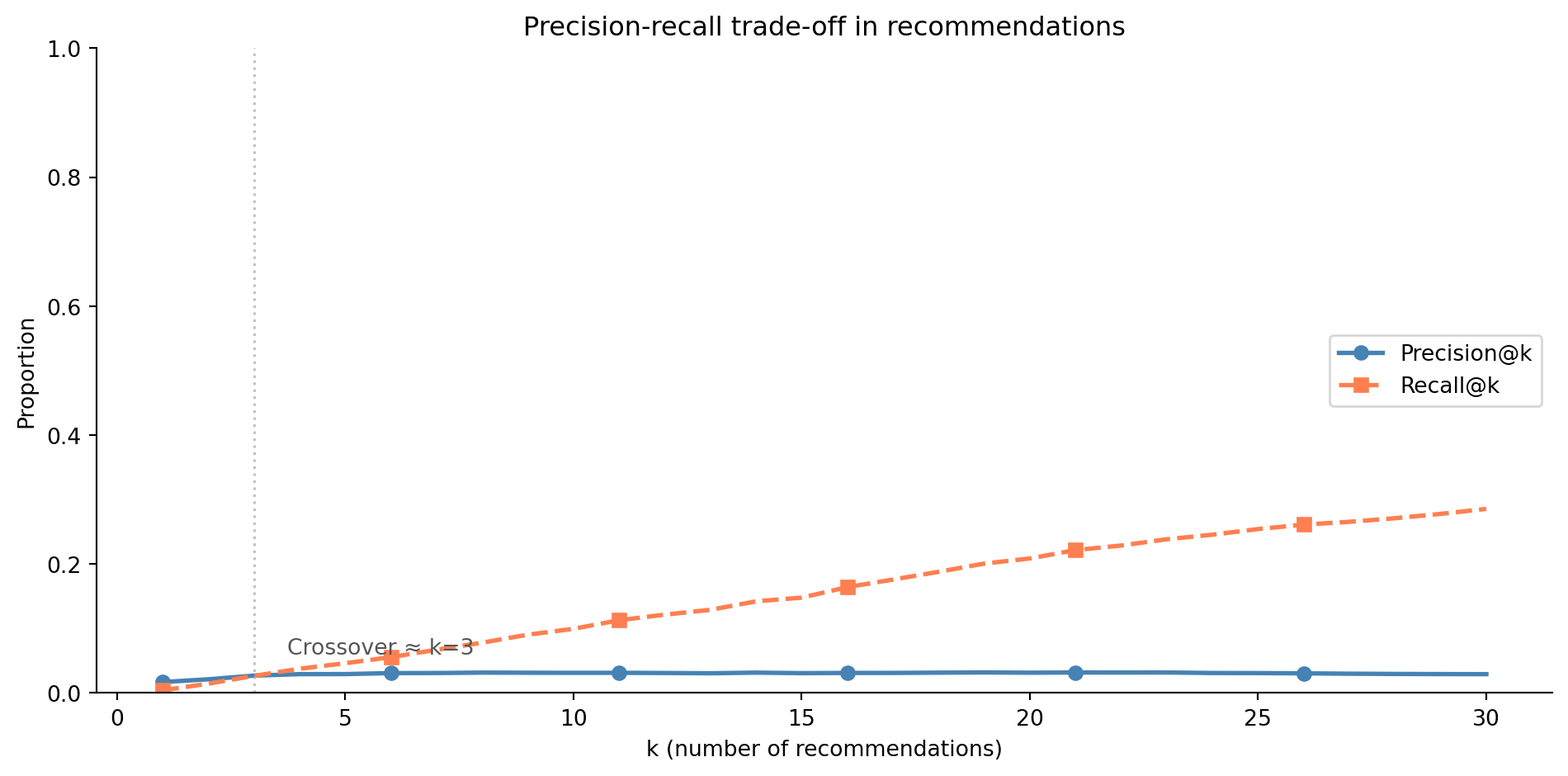
**Precision@k** asks: of the $k$ items recommended, how many were relevant (the fraction of true positives among recommendations)? **Recall@k** asks: of all relevant items, how many appeared in the top $k$? These are the same precision and recall concepts from @sec-precision-recall-tradeoff, adapted for ranked lists rather than binary classification. A third common metric, **normalised discounted cumulative gain** (NDCG), also accounts for the *position* of relevant items: a relevant item at position 1 matters more than one at position 10.
```{python}
#| label: fig-k-tradeoff
#| echo: true
#| fig-cap: "Precision@k and Recall@k as a function of k. As k increases, recall improves (more relevant items are surfaced) but precision declines (more irrelevant items dilute the list). The dashed vertical line marks the crossover point where the two curves meet."
#| fig-alt: "Line chart with two curves showing how precision and recall change as the number of recommendations k increases from 1 to 30. The precision@k curve (solid line with circle markers) falls as more items are recommended. The recall@k curve (dashed line with square markers) rises from near zero. A vertical dashed line marks the crossover point where precision and recall are equal, illustrating the precision-recall trade-off in ranked recommendation lists."
ks = list(range(1, 31))
precs, recs = [], []
for k in ks:
    p, r = evaluate_precision_recall_at_k(
        test_df, train_matrix, train_item_sim, k=k
    )
    precs.append(p)
    recs.append(r)

fig, ax = plt.subplots(figsize=(10, 5))
fig.patch.set_alpha(0)
ax.patch.set_alpha(0)
ax.plot(ks, precs, color='#0072B2', linewidth=2, linestyle='-',
        marker='o', markevery=5, label='Precision@k')
ax.plot(ks, recs, color='#E69F00', linewidth=2, linestyle='--',
        marker='s', markevery=5, label='Recall@k')

# Mark the crossover point
cross_idx = np.argmin(np.abs(np.array(precs) - np.array(recs)))
ax.axvline(ks[cross_idx], color='#aaaaaa', linestyle=':', linewidth=1.2, alpha=0.7)
ax.annotate(f'Crossover ≈ k={ks[cross_idx]}',
            xy=(ks[cross_idx], precs[cross_idx]),
            xytext=(15, 10), textcoords='offset points',
            fontsize=10, color='#555555')

ax.set_xlabel('k (number of recommendations)')
ax.set_ylabel('Proportion')
ax.set_ylim(0, 0.45)
ax.set_title('Precision-recall trade-off in recommendations')
ax.legend(loc='center right')
ax.spines[['top', 'right']].set_visible(False)
plt.tight_layout()
plt.show()
```
But even these metrics miss something important. A recommendation system that only surfaces safe, popular choices might score well on precision but feel generic and unhelpful. Good recommendations balance **relevance** (items the user would rate highly), **novelty** (items the user hasn't already discovered), and **diversity** (variety across the recommended list). These qualities are harder to measure offline and often require online A/B testing (@sec-ab-testing), showing real users different recommendation strategies and measuring engagement.
Offline evaluation has a deeper limitation: the test set only contains items users chose to interact with. Users who were already guided by a recommendation system had their choices shaped by it, a form of **exposure bias** (technically, the missing data is not missing at random). High precision on held-out ratings tells you the model is good at predicting preferences for items users were already inclined to discover; it tells you nothing about whether the system would surface items the user didn't know they wanted. This is why online experimentation remains essential.
Recommendation systems also create **feedback loops**. Popular items get recommended more often, which generates more interactions, which makes them appear even more popular. Over time, this concentrates attention on a shrinking set of items while the long tail becomes invisible. Strategies like reserving exploration slots for new or underrepresented items, applying inverse propensity weighting, and enforcing diversity constraints can counteract this, but you need to measure the effect explicitly (catalogue coverage, Gini coefficient of item exposure) rather than assuming the feedback loop is benign.
## Implicit feedback: when you don't have ratings {#sec-implicit-feedback}
We've been working with explicit ratings: users telling us how much they liked something on a scale of 1 to 5. Most real-world systems don't have this luxury. Instead, they observe **implicit feedback**: clicks, purchases, time spent, pages scrolled, items added to a basket and later abandoned. These signals are abundant but ambiguous. A user clicking on an item might mean genuine interest, an accidental tap, or morbid curiosity. Not clicking doesn't mean dislike — the user may simply not have seen it.
Explicit feedback has both positive and negative signals: ratings of 1 and 5 are both informative. Implicit feedback is **one-class**: you observe what users did but not what they deliberately chose to avoid. This changes the modelling approach. Instead of predicting a rating, you predict a **preference probability** and weight it by a **confidence** derived from the interaction strength [@hu2008].
```{python}
#| label: implicit-feedback
#| echo: true
# Simulate implicit feedback: view counts instead of ratings
implicit_df = ratings_df.copy()
# Convert ratings to "interaction strength" (e.g., number of times viewed)
implicit_df['views'] = (implicit_df['rating'] * rng.poisson(3, len(implicit_df))
                        + rng.poisson(1, len(implicit_df)))
implicit_df = implicit_df.drop(columns=['rating'])

# In implicit feedback, confidence increases with interaction strength.
# The standard formulation uses c_ui = 1 + alpha_conf * views, where alpha_conf
# is a confidence scaling parameter (distinct from the blending weight in
# the hybrid recommender above).
alpha_conf = 40
implicit_df['confidence'] = 1 + alpha_conf * implicit_df['views']
implicit_df['preference'] = 1  # all observed interactions are positive

print('Implicit feedback sample:')
print(implicit_df.head(10).to_string(index=False))
print(f"\nConfidence range: [{implicit_df['confidence'].min()}, "
      f"{implicit_df['confidence'].max()}]")
```
The confidence-weighted approach (with $\alpha_\text{conf}$ as a hyperparameter you'd tune empirically; values in the literature range from 1 to 40 depending on the domain) treats every observed interaction as a positive signal with varying strength, and every *unobserved* interaction as a weak negative. A user who watched a film five times gives a stronger positive signal than one who watched thirty seconds and moved on, but both are positive, and neither is as informative as a user explicitly rating something one star.
::: {.callout-tip}
## Author's Note
The shift from explicit to implicit feedback changed my understanding of what recommendation systems actually do. With ratings, you're solving a regression problem, i.e., predict the number. With implicit data, you're solving something closer to an information retrieval problem, i.e., rank the items the user would engage with above the ones they wouldn't. This distinction matters because the loss function, the evaluation metrics, and the baseline expectations all change. Accuracy on a 1–5 scale is meaningless when your data is binary clicks. It's a reminder that the framing of the problem shapes everything downstream, a lesson that applies well beyond recommendation systems.
:::
## Scaling recommendations {#sec-recsys-scaling}
A recommendation system that takes ten seconds to generate results is useless in production, regardless of its accuracy. The scaling challenges are twofold: **offline computation** (training models and precomputing scores) and **online serving** (generating personalised recommendations at request time with low latency).
For collaborative filtering, the item-item similarity matrix is $O(n^2)$ in items, manageable for thousands of items, prohibitive for millions. Matrix factorisation scales better: once you've learned the latent factors, generating a single user's recommendations is a dot product over $K$ dimensions, which is fast.
The standard production pattern is to precompute recommendations in a batch job (nightly or hourly), store the top-$k$ items per user in a fast key-value store, and serve them directly on request. For users who need real-time adaptation (they just bought something), a lightweight re-ranking layer adjusts the precomputed list based on the latest interaction, removing items similar to what was just purchased and boosting items in related categories.
Note that precomputation and model retraining operate on different schedules. You might recompute the top-$k$ lists hourly (cheap — just matrix multiplication and sorting), but retrain the latent factor model weekly or monthly (expensive — full optimisation pass over all observed interactions). Serving stale lists from a fresh model is different from serving fresh lists from a stale model; monitoring both cadences matters.
```{python}
#| label: scaling-precompute
#| echo: true
import time

# Demonstrate precomputation: generate top-10 recommendations for all users.
# This materialises the full score matrix — feasible at our demo scale (500×200)
# but not at production scale with millions of users and items. At scale, you'd
# use approximate nearest neighbour (ANN) libraries (e.g. Faiss, Annoy, ScaNN)
# to find the top-k items in latent space without computing all pairwise scores.
start = time.perf_counter()

all_scores = user_latent @ item_latent.T  # (n_users, n_items)

# Mask already-rated items
dense_interactions = interaction_matrix.toarray()
all_scores[dense_interactions > 0] = -np.inf

# Top-k per user
k = 10
top_k_items = np.argsort(all_scores, axis=1)[:, -k:][:, ::-1]

elapsed = time.perf_counter() - start
print(f"Precomputed top-{k} for {n_users} users in {elapsed*1000:.1f}ms")
print(f"Storage: {top_k_items.nbytes / 1024:.1f} KB for the lookup table")
print(f"\nUser 0 precomputed recommendations: {top_k_items[0]}")
```
The precomputation is fast for our 500-user demonstration dataset, but the full score matrix grows as $O(\text{users} \times \text{items})$, so it doesn't scale to millions. The engineering patterns from @sec-scale-intro (chunked processing, vectorisation, and choosing the right data structure) apply directly to the batch scoring job, while approximate nearest neighbour (ANN) libraries handle the nearest-neighbour search in latent space.
At the largest scale, neural approaches (two-tower models and transformer-based sequence recommenders) have largely supplanted matrix factorisation, at the cost of significantly more training infrastructure. The principles are the same (learn latent representations, score via dot products, serve via ANN search), but the representation learning is deeper. Those architectures are beyond our scope here; the matrix factorisation framework gives you the conceptual foundation they build on.
::: {.callout-note}
## Engineering Bridge
The precompute-and-serve pattern maps directly to the cache-aside architecture common in web services. You compute the expensive operation asynchronously (model training and score generation), store the results in a fast-access layer (Redis, Memcached, or a purpose-built feature store), and serve requests from the cache. Cache invalidation — the "hardest problem in computer science" — has a direct analogue: when should you recompute recommendations? After every interaction (expensive but fresh), on a schedule (cheap but stale), or on a hybrid trigger (recompute when the user's interaction count crosses a threshold)? The trade-offs are identical to those in any caching system. One additional wrinkle: a user exercising their right to erasure under GDPR doesn't just remove a row from the interaction table; their preferences are encoded in the model's latent factors. Full compliance may require retraining the model after deletion, not just clearing the cache.
:::
## From predicted scores to delivered recommendations {#sec-from-scores-to-delivery}
Everything so far has produced *scores*: real-valued estimates of how much a given user would like a given item. A production system has to turn those scores into a concrete list shown on a screen, and that translation involves three product decisions that look like engineering choices but aren't.
*List size is a product constraint, not an optimum.* The precision-recall trade-off in @fig-k-tradeoff might suggest that *k* = 12 is the offline sweet spot, but the homepage carousel shows six tiles, the email digest has space for three, and the mobile push notification carries one. You pick *k* to match the slot, then choose the model and ranking that maximise the metric *at that k*. Going the other way — picking the statistically optimal *k* and asking the product team to redesign around it — does not happen.
*Retrieval and ranking are two stages with different jobs.* At catalogue sizes above a few tens of thousands of items, you cannot score every item for every user on every request. The standard pattern is a two-stage funnel. **Retrieval** narrows the catalogue from millions of items to a few hundred candidates per user, using fast approximate methods: nearest-neighbour lookup over latent factors, popularity baselines, recently-trending items, and content-based filters. **Ranking** then re-scores those few hundred candidates with a heavier model that can afford richer features (recency, session context, business-rule overrides). The retrieval stage optimises for *recall* — make sure the relevant items survive — because anything cut here cannot be ranked. The ranking stage optimises for *ordering* — get the best item to the top.
```{python}
#| label: retrieve-then-rank
#| echo: true
# Two-stage funnel: cheap retrieval narrows the catalogue,
# heavier ranking orders what survives. In production, n_candidates
# is typically 100-1000 drawn from a catalogue of millions; here we
# use 50 from our 200-item toy catalogue to show the shape of the
# computation.
def retrieve_and_rank(user_id, user_latent, item_latent, n_candidates=50, top_k=10):
    # Stage 1: retrieve top-N candidates by latent-factor dot product (fast)
    user_vec = user_latent[user_id]
    candidate_scores = item_latent @ user_vec
    # argpartition requires kth < len(a); clip to keep the function robust
    # on small catalogues like this one
    kth = min(n_candidates, len(candidate_scores) - 1)
    candidate_idx = np.argpartition(-candidate_scores, kth)[:n_candidates]

    # Stage 2: re-rank candidates with richer signals (here just popularity prior;
    # in production: recency, session features, business overrides, A/B variants).
    item_popularity = (interaction_matrix > 0).sum(axis=0).A1
    rerank = candidate_scores[candidate_idx] + 0.1 * np.log1p(item_popularity[candidate_idx])
    final_order = candidate_idx[np.argsort(-rerank)[:top_k]]
    return final_order

print(f"Two-stage recommendations for user 0: {retrieve_and_rank(0, user_latent, item_latent)}")
```
The two stages also have different latency budgets and different evaluation metrics. Recall@$N$ (where $N$ is the candidate-set size) is what you measure for the retrieval stage; NDCG@$k$ (where $k$ is the number of items shown to the user) is what you measure for the ranking stage. Conflating them — using the same metric for both — wastes engineering effort on the wrong stage.
*Offline metrics are a proxy; the real evaluation is online.* This is the load-bearing point of the chapter and worth saying plainly. Precision@k, recall@k, NDCG, hit rate, MRR — every offline metric is computed against the data your *previous* recommender produced, which means it can only score how well a new system mimics or modestly improves on the patterns the old system created. It cannot tell you whether the new system surfaces items users would have loved but never saw. The verdict on user impact comes from an A/B test (see @sec-ab-testing) measuring engagement, conversion, retention, or revenue against a control group on real traffic.
What does that leave offline metrics good for? Quite a lot, actually — but the boundary is sharp:
| Offline metrics are useful for | Offline metrics cannot tell you |
| --: | :-- |
| Comparing model architectures during iteration | Whether real users will engage with the recommendations |
| Catching regressions before they reach production | Effects of novelty, freshness, or surprise |
| Tuning hyperparameters cheaply | Long-term retention or business outcomes |
| Sanity-checking that a model has learned anything | The impact of the recommendation on user behaviour (the loop @sec-recsys-evaluation describes) |
| Establishing minimum quality gates for promotion | Cross-product effects (does ranking change browsing patterns?) |
: When to trust offline metrics — and when to reach for an A/B test. {#tbl-offline-vs-online}
The practical workflow is to use offline metrics as a fast gate (does this model regress? does it match the baseline?) and to reserve A/B testing for the actual go/no-go decision. A model that improves NDCG by 5% offline might lose to the incumbent on click-through rate online. A model that ties the incumbent offline might win decisively on retention. Until you ship, you do not know.
## Summary {#sec-recsys-summary}
1. **Recommendation is a missing-data problem.** The interaction matrix is overwhelmingly sparse, and the core challenge is predicting the missing entries — what would each user think of items they haven't seen?
2. **Collaborative filtering works from behaviour, not features.** It exploits the observation that users who agreed in the past tend to agree in the future. Item-based and user-based variants differ in which axis of the matrix they compute similarity over.
3. **Matrix factorisation compresses the interaction matrix into latent factors.** By forcing ratings through a low-dimensional bottleneck, it learns the underlying structure of preferences and generalises across sparse observations — the same principle as PCA applied to a matrix with missing values.
4. **Content-based filtering uses item features to bridge the cold-start gap.** New items without ratings can still be recommended based on their attributes. Hybrid systems combine collaborative and content-based signals for robustness.
5. **Evaluation requires ranking metrics, not just prediction error.** Precision@k, Recall@k, and NDCG measure whether the system surfaces relevant items in the top positions. Online A/B testing remains essential because offline metrics don't capture novelty, diversity, or user satisfaction.
6. **Production recommendation is a two-stage funnel, and offline metrics are a proxy.** Retrieval narrows the catalogue; ranking orders the survivors; list size is set by the product surface, not the precision-recall curve. Use offline metrics as a fast gate during iteration and reserve A/B testing for the actual go/no-go decision on user impact.
## Exercises {#sec-recsys-exercises}
1. Implement **user-based** collaborative filtering by computing cosine similarity between user rows (instead of item columns) of the interaction matrix. Compare its recommendations for user 0 with the item-based approach from @sec-collaborative-filtering. Under what conditions would you expect user-based to outperform item-based, and vice versa?
2. The hybrid recommender in @sec-hybrid uses a fixed blending weight $w = 0.6$ (the `w` parameter in the code). Split the training data further into train and validation subsets (80/20), then write a function that tunes $w$ by evaluating precision@10 on the validation set for values of $w$ from 0 to 1 in steps of 0.1. Plot precision@10 as a function of $w$. Is the optimal blend closer to pure collaborative or pure content-based?
3. **Evaluating diversity.** Write a function that computes the **intra-list diversity** of a recommendation list — the average pairwise distance (1 minus cosine similarity) between the recommended items' content features. Compute this metric for the collaborative, content-based, and hybrid recommenders. Which produces the most diverse recommendations? Why?
4. **Conceptual:** A product manager proposes using purchase history as the sole input for recommendations on an e-commerce site. What signals would this miss compared to using browsing behaviour (page views, search queries, time on page)? What are the risks of including browsing behaviour — when might a signal be misleading?
5. **Conceptual:** Recommendation systems create feedback loops — popular items get recommended more often, which generates more interactions, which makes them appear even more popular. How does this **popularity bias** affect the system over time? What mechanisms could you introduce to ensure that new or niche items still get discovered? How would you measure whether your intervention is working?