---
# Content: CC BY-NC-SA 4.0 | Code: MIT - see /LICENSE.md
title: "Confidence intervals: error bounds for estimates"
---
{{< include /_common-imports.qmd >}}
## Every estimate needs an error bar {#sec-confidence-intervals}
When you profile a function and your tool reports "mean execution time: 42ms," you don't take that number at face value. You know it depends on how many times you ran the function, what else was running on the machine, and whether the JIT compiler had warmed up. The single number is useful, but what you really want is a *range* — "42ms, give or take 3ms" — that tells you how much to trust it.
That's what a confidence interval is: a range around an estimate that quantifies its uncertainty. We built the machinery for this in @sec-standard-error and @sec-clt: the standard error measures the precision of an estimate, and the Central Limit Theorem (CLT) tells us the sampling distribution is approximately Normal. A confidence interval translates those ingredients into a statement the reader can act on: "the true value is plausibly between here and here."
## Constructing a confidence interval for the mean {#sec-ci-construction}
Suppose you sample 100 API response times and get a mean of 54.2ms with a standard deviation of 18ms. In @sec-testing-framework, we used these numbers to test whether the mean had shifted from 50ms. Now we'll use them to build an interval that captures the plausible range of the true mean.
The logic starts with the sampling distribution. By the CLT (which assumes the population has finite variance), $\bar{X}$ (the sample mean, viewed as a random variable that varies from sample to sample) is approximately Normal with mean $\mu$ (the true population mean) and standard error $\sigma / \sqrt{n}$, which we estimate from the data as $s / \sqrt{n}$. This means that about 95% of the time, the sample mean will land within roughly 2 standard errors of $\mu$, and by symmetry, $\mu$ will land within roughly 2 standard errors of $\bar{X}$.
The "roughly 2" is more precisely $z^* = 1.96$, the **critical value** for a 95% interval. A critical value is the threshold on the reference distribution that cuts off the desired tail probability; here, $z^* = 1.96$ leaves 2.5% in each tail of the standard Normal (the Normal distribution with mean 0 and standard deviation 1). For smaller samples, we use $t^*$ from the t-distribution instead, which has heavier tails (more probability in the extremes) that account for the extra uncertainty from estimating the population standard deviation $\sigma$ with the sample standard deviation $s$. The subscript in $t^*_{n-1}$ denotes the degrees of freedom ($n - 1$ for a single-sample mean). At $n = 100$ the difference is small ($t^*_{99} \approx 1.984$ vs $z^* = 1.960$), but for $n = 15$ it matters.
$$
\text{CI} = \bar{x} \;\pm\; t^*_{n-1} \times \frac{s}{\sqrt{n}}
$$
In words: the sample mean, plus or minus a critical value times the standard error.
```{python}
#| label: ci-construction
#| echo: true
from scipy import stats

# Same summary statistics as our SLO test in the previous chapter
sample_mean = 54.2
sample_std = 18.0
n = 100

# Standard error
se = sample_std / np.sqrt(n)

# 95% confidence interval using the t-distribution
confidence_level = 0.95
# ppf = percent point function (inverse CDF): returns the t-value below which
# a given fraction of the distribution falls.
# (1 + 0.95) / 2 = 0.975 — we want the value that leaves 2.5% in each tail
t_crit = stats.t.ppf((1 + confidence_level) / 2, df=n - 1)

ci_lower = sample_mean - t_crit * se
ci_upper = sample_mean + t_crit * se

print(f"Sample mean: {sample_mean} ms")
print(f"Standard error: {se:.2f} ms")
print(f"t* (df={n-1}): {t_crit:.3f}")
print(f"95% CI: ({ci_lower:.1f}, {ci_upper:.1f}) ms")
print(f"\nWe estimate the true mean response time is between "
      f"{ci_lower:.1f} ms and {ci_upper:.1f} ms.")
```
The interval (50.6, 57.8) tells us something the p-value from @sec-testing-framework didn't: not just that the mean has shifted, but by *how much* it plausibly shifted. The SLO (service-level objective) target of 50ms falls outside this interval, which is consistent with rejecting $H_0$ (the null hypothesis, "nothing has changed"), and that's not a coincidence, as we'll see in @sec-ci-test-duality.
Let's verify with `scipy`'s built-in method. Since we're working from summary statistics rather than raw data, we'll pass those directly to `stats.t.interval`.
```{python}
#| label: ci-scipy-verify
#| echo: true
# Verify using scipy — pass summary statistics directly
# loc = centre of the distribution (sample mean)
# scale = spread (standard error)
ci = stats.t.interval(0.95, df=n - 1,
                       loc=sample_mean,
                       scale=se)

print(f"scipy 95% CI: ({ci[0]:.1f}, {ci[1]:.1f}) ms")
```
## What the confidence level actually means {#sec-ci-interpretation}
The 95% in "95% confidence interval" is the most misunderstood number in statistics, rivalling the p-value for how often it's explained incorrectly.
**It does not mean:** "there is a 95% probability that the true mean lies in this interval." Once you've computed the interval, the true mean either is in it or it isn't; there's no probability involved for that specific interval.
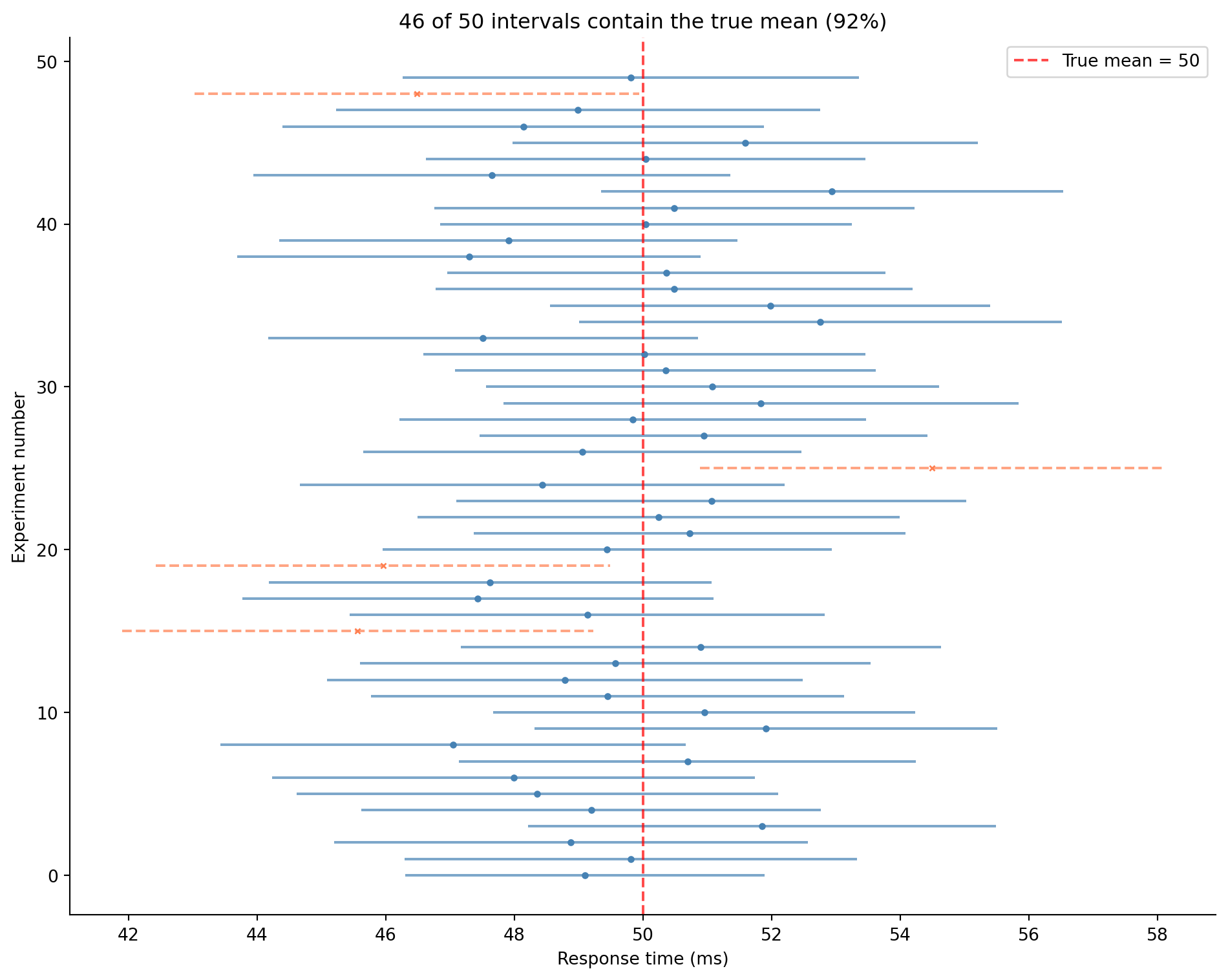
**It does mean:** if you repeated the experiment many times, each time computing a new 95% confidence interval (CI) from a fresh sample, about 95% of those intervals would contain the true mean. @fig-ci-simulation makes this concrete.
The confidence level describes the *procedure*, not any single interval. "95% confidence" tells you that the procedure captures the true value in 95% of repetitions, not whether this particular interval got lucky.
```{python}
#| label: fig-ci-simulation
#| echo: true
#| fig-cap: "500 confidence intervals from repeated sampling, each a fresh 95% CI from a new sample. The solid intervals capture the true mean (dashed vertical line); the dashed ones (× markers) miss. Over many repetitions the capture rate approaches 95% — with a finite number it varies around that value, as the title for this run shows."
#| fig-alt: "Horizontal line segments representing 500 confidence intervals stacked vertically into a dense band. The large majority are solid blue lines crossing the vertical dotted true-mean line at 50ms; a minority are dashed orange lines with cross markers, indicating they missed. The chart title reports the number and percentage of intervals that captured the true mean, close to the nominal 95%."
rng = np.random.default_rng(10)

true_mean = 50
true_std = 18
n = 100
n_experiments = 500

fig, ax = plt.subplots(figsize=(10, 8))
fig.patch.set_alpha(0)
ax.patch.set_alpha(0)

contains_true = 0
for i in range(n_experiments):
    sample = rng.normal(true_mean, true_std, n)
    x_bar = sample.mean()
    # ddof=1: divide by n-1 (Bessel's correction) for unbiased SD estimate
    se = sample.std(ddof=1) / np.sqrt(n)
    t_crit = stats.t.ppf(0.975, df=n - 1)

    lower = x_bar - t_crit * se
    upper = x_bar + t_crit * se

    captured = lower <= true_mean <= upper
    if captured:
        contains_true += 1
    colour = '#0072B2' if captured else '#E69F00'
    ls = '-' if captured else '--'
    marker = 'o' if captured else 'x'

    ax.plot([lower, upper], [i, i], color=colour, linestyle=ls,
            linewidth=0.8, alpha=0.6)
    ax.plot(x_bar, i, marker, color=colour, markersize=2)

ax.axvline(true_mean, color='#444', linestyle=':', linewidth=1.5,
           label=f'True mean = {true_mean}')
ax.set_xlabel('Response time (ms)')
ax.set_ylabel('Experiment number')
ax.set_title(f'{contains_true} of {n_experiments} intervals contain the true mean '
             f'({contains_true/n_experiments:.0%})')
ax.legend()
ax.spines[['top', 'right']].set_visible(False)
plt.tight_layout()
plt.show()
```
With a finite number of repetitions the observed capture rate fluctuates around the nominal 95% rather than landing on it exactly; the title reports the rate for this particular run. Run the experiment enough times and it converges to almost precisely 95% — that convergence *is* the guarantee the confidence level makes. A few hundred repetitions are enough to see the pattern, not to pin the rate to the decimal.
::: {.callout-tip}
## Author's Note
The standard misreading of confidence intervals, "95% chance the true value is in here," *feels* like the natural interpretation. What makes it wrong is subtle: the procedure's guarantee is about the *long-run hit rate*, not about any single interval. Think of it like a P95 latency SLA: "our P95 is under 100ms" is a statement about the distribution of the process, not about any one request. Similarly, "95% confidence" tells you that the interval-construction procedure captures the true value 95% of the time, not that this particular interval has a 95% probability of being correct. The confidence level is a property of the method, not of the result.
:::
## Confidence interval for a proportion {#sec-ci-proportion}
In @sec-two-sample-test, we tested whether the A/B test conversion rates were significantly different and concluded there wasn't enough evidence. A confidence interval tells us something richer: what range of true differences is consistent with the data?
For a proportion, where $\hat{p}$ ("p-hat") is the observed sample proportion, the standard error is $\sqrt{\hat{p}(1 - \hat{p}) / n}$, and the CI follows the same pattern:
$$
\text{CI} = \hat{p} \;\pm\; z^* \times \sqrt{\frac{\hat{p}(1 - \hat{p})}{n}}
$$
In words: the observed proportion, plus or minus a critical value times its standard error. This is the **Wald interval**, the simplest CI for a proportion, built directly from the Normal approximation. It works well when $n\hat{p}$ and $n(1 - \hat{p})$ are both comfortably large (here, $n\hat{p} = 120$). When $p$ is near 0 or 1, or $n$ is small, the Wald interval can have poor **coverage**: the actual fraction of intervals that contain the true value (as @fig-ci-simulation demonstrated) drops well below the nominal 95%. In practice, the **Wilson interval** is the better default for proportions; it maintains accurate coverage across a much wider range of $n$ and $p$. At these sample sizes the two give near-identical results, which is why we show the simpler Wald interval here.
We use $z^*$ (the Normal critical value) rather than $t^*$ here. The Wald interval relies on the large-sample Normal approximation to the sampling distribution of $\hat{p}$, so the standard Normal is the right reference distribution. There is no exact small-sample t analogue for a proportion: the t-distribution arises specifically from estimating $\sigma$ for a Normal mean, and switching to it would not fix the failure mode that matters here. (The Wald SE *is* estimated — we plug $\hat{p}$ into $\sqrt{\hat{p}(1-\hat{p})/n}$ — so there is estimation uncertainty; it just isn't the kind the t correction addresses.) That reliance on the Normal approximation is precisely why the Wald interval degrades for small $n$ or extreme $p$, which is the motivation for the Wilson interval mentioned above.
One subtlety: when we tested these proportions in @sec-two-sample-test, we used a **pooled** standard error (combining both groups) because $H_0$ assumed the rates were equal. For the CI, we don't assume equality; we're estimating the actual difference. So each group keeps its own SE (unpooled).
```{python}
#| label: ci-proportions
#| echo: true
# A/B test data from the previous chapters
n_control, n_variant = 1000, 1000
p_control, p_variant = 0.120, 0.135

z_crit = stats.norm.ppf(0.975)  # 0.975 = 1 - 0.05/2; leaves 2.5% in each tail → 1.96

# CI for each group
se_control = np.sqrt(p_control * (1 - p_control) / n_control)
se_variant = np.sqrt(p_variant * (1 - p_variant) / n_variant)

ci_control = (p_control - z_crit * se_control, p_control + z_crit * se_control)
ci_variant = (p_variant - z_crit * se_variant, p_variant + z_crit * se_variant)

print(f"Control: {p_control:.1%}  95% CI: ({ci_control[0]:.1%}, {ci_control[1]:.1%})")
print(f"Variant: {p_variant:.1%}  95% CI: ({ci_variant[0]:.1%}, {ci_variant[1]:.1%})")

# CI for the difference — unpooled SEs (see prose above)
diff = p_variant - p_control
se_diff = np.sqrt(se_control**2 + se_variant**2)
ci_diff = (diff - z_crit * se_diff, diff + z_crit * se_diff)

print(f"\nDifference: {diff:.1%}")
print(f"95% CI for difference: ({ci_diff[0]:.1%}, {ci_diff[1]:.1%})")
print(f"\nThe interval includes zero, consistent with our earlier failure to reject H₀.")
```
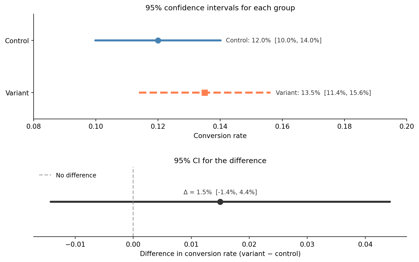
@fig-ci-ab-test visualises these intervals. The confidence interval for the difference ranges from about −1.4 to +4.4 percentage points. Because it includes zero, we can't rule out "no effect", which aligns with the non-significant p-value from @sec-two-sample-test. But the interval also includes differences as large as 4.4 percentage points, which would be substantial. The CI tells us that we lack *precision*, not that the effect is small.
```{python}
#| label: fig-ci-ab-test
#| echo: true
#| fig-cap: "Confidence intervals for control and variant conversion rates (top panel) and for their difference (bottom panel). The difference CI includes zero, so we cannot claim significance."
#| fig-alt: "Two-panel figure. The top panel shows horizontal CI lines for control (solid blue, 12.0% with CI 10.0–14.0%) and variant (dashed orange, 13.5% with CI 11.4–15.6%), with their intervals overlapping substantially. The bottom panel shows the CI for the difference centred near 1.5 percentage points, with a dashed vertical line at zero falling well within the interval, indicating we cannot rule out no effect."
lower_diff, upper_diff = ci_diff

fig, (ax1, ax2) = plt.subplots(
    2, 1, figsize=(10, 6),
    gridspec_kw={'height_ratios': [3, 2], 'hspace': 0.55},
)
fig.patch.set_alpha(0)
ax1.patch.set_alpha(0)
ax2.patch.set_alpha(0)

# ── Top: individual group CIs ──
groups = [
    (1, p_control, se_control, 'Control', '#0072B2', '-', 'o'),
    (0, p_variant, se_variant, 'Variant', '#E69F00', '--', 's'),
]
for y, p, se, label, colour, ls, marker in groups:
    lo = p - z_crit * se
    hi = p + z_crit * se
    ax1.plot([lo, hi], [y, y], color=colour, linestyle=ls,
             linewidth=3, solid_capstyle='round')
    ax1.plot(p, y, marker, color=colour, markersize=8, zorder=5)
    ax1.annotate(
        f'{label}: {p:.1%}  [{lo:.1%}, {hi:.1%}]',
        xy=(hi, y), xytext=(8, 0), textcoords='offset points',
        fontsize=9, va='center', color='#333',
    )

ax1.set_yticks([0, 1])
ax1.set_yticklabels(['Variant', 'Control'])
ax1.set_xlabel('Conversion rate')
ax1.set_title('95% confidence intervals for each group', fontsize=11)
ax1.set_xlim(0.08, 0.20)
ax1.set_ylim(-0.5, 1.5)
ax1.spines[['top', 'right']].set_visible(False)

# ── Bottom: CI for the difference ──
ax2.plot([lower_diff, upper_diff], [0, 0], color='#333', linewidth=3,
         solid_capstyle='round')
ax2.plot(diff, 0, 'o', color='#333', markersize=8, zorder=5)
ax2.axvline(0, color='grey', linestyle='--', alpha=0.6, label='No difference')
ax2.annotate(
    f'Δ = {diff:.1%}  [{lower_diff:.1%}, {upper_diff:.1%}]',
    xy=(diff, 0), xytext=(0, 12), textcoords='offset points',
    fontsize=9, ha='center', color='#333',
)

ax2.set_xlabel('Difference in conversion rate (variant − control)')
ax2.set_title('95% CI for the difference', fontsize=11)
ax2.set_ylim(-0.6, 0.6)
ax2.set_yticks([])
ax2.spines[['top', 'right', 'left']].set_visible(False)
ax2.legend(loc='upper left', fontsize=9, frameon=False)

plt.tight_layout()
plt.show()
```
::: {.callout-note}
## Engineering Bridge
Think of confidence intervals as **error bounds**, the same concept you use in numerical computing and systems design. When a load balancer reports "average latency: 42ms ± 3ms," the ± is doing the same job as a confidence interval: it tells you how much the estimate might move if you measured again. The CI width is the *tolerance* on your measurement. A narrow CI means high precision; you can confidently act on the number. A wide CI means the measurement is noisy and you need more data (or a better measurement process) before making a decision. In A/B testing, this matters directly: a CI of (−1.4 pp, +4.4 pp) is too wide to act on in either direction.
:::
## The duality: tests and intervals are two views of the same thing {#sec-ci-test-duality}
There's a deep connection between confidence intervals and hypothesis tests. Rejecting $H_0$ at significance level $\alpha$ is *equivalent* to the hypothesised value falling outside the $(1 - \alpha)$ confidence interval. (This duality holds for two-sided tests and two-sided intervals at matching levels. For one-sided tests, the analogue is a one-sided confidence bound: "the true mean is at most X.")
In our SLO example from @sec-testing-framework, the 95% CI for the mean response time was (50.6, 57.8). The hypothesised value of 50ms falls outside this interval, so we reject $H_0: \mu = 50$ at $\alpha = 0.05$. The two procedures always agree.
```{python}
#| label: ci-test-duality
#| echo: true
# From the SLO test in the previous chapter
sample_mean = 54.2
sample_std = 18.0
n = 100
hypothesised_mean = 50.0

se = sample_std / np.sqrt(n)
t_crit = stats.t.ppf(0.975, df=n - 1)

# Confidence interval
ci_lower = sample_mean - t_crit * se
ci_upper = sample_mean + t_crit * se

# Hypothesis test
t_stat = (sample_mean - hypothesised_mean) / se
# sf = survival function = P(T > t), i.e. 1 - CDF; ×2 for two-sided test
p_value = 2 * stats.t.sf(abs(t_stat), df=n - 1)

print(f"95% CI: ({ci_lower:.1f}, {ci_upper:.1f})")
print(f"H₀: μ = {hypothesised_mean}")
print(f"Is {hypothesised_mean} inside the CI? {ci_lower <= hypothesised_mean <= ci_upper}")
print(f"\np-value: {p_value:.4f}")
print(f"Reject H₀ at α = 0.05? {p_value < 0.05}")
print(f"\nBoth methods agree: the test rejects and the CI excludes 50.")
```
So why use CIs at all, if they give the same binary answer? Because the CI gives you *more* information. The p-value tells you *whether* to reject: the mean has shifted. The CI tells you *where* the true value plausibly lies: between 50.6 and 57.8ms. That range is what you need to make a decision: is a 1–8 ms increase worth investigating?
This is why many journals and style guides now recommend reporting CIs alongside (or instead of) p-values. A CI communicates effect size (the magnitude of the difference) and precision in a single object. We'll rely on this duality when we design A/B tests in *A/B testing: deploying experiments*. And if the frequentist interpretation feels unsatisfying — if what you really want is "there's a 95% probability the true value is in this range" — that's exactly what a Bayesian **credible interval** provides. We'll build one in *Bayesian inference: updating beliefs with evidence*.
## What makes intervals wider or narrower {#sec-ci-width}
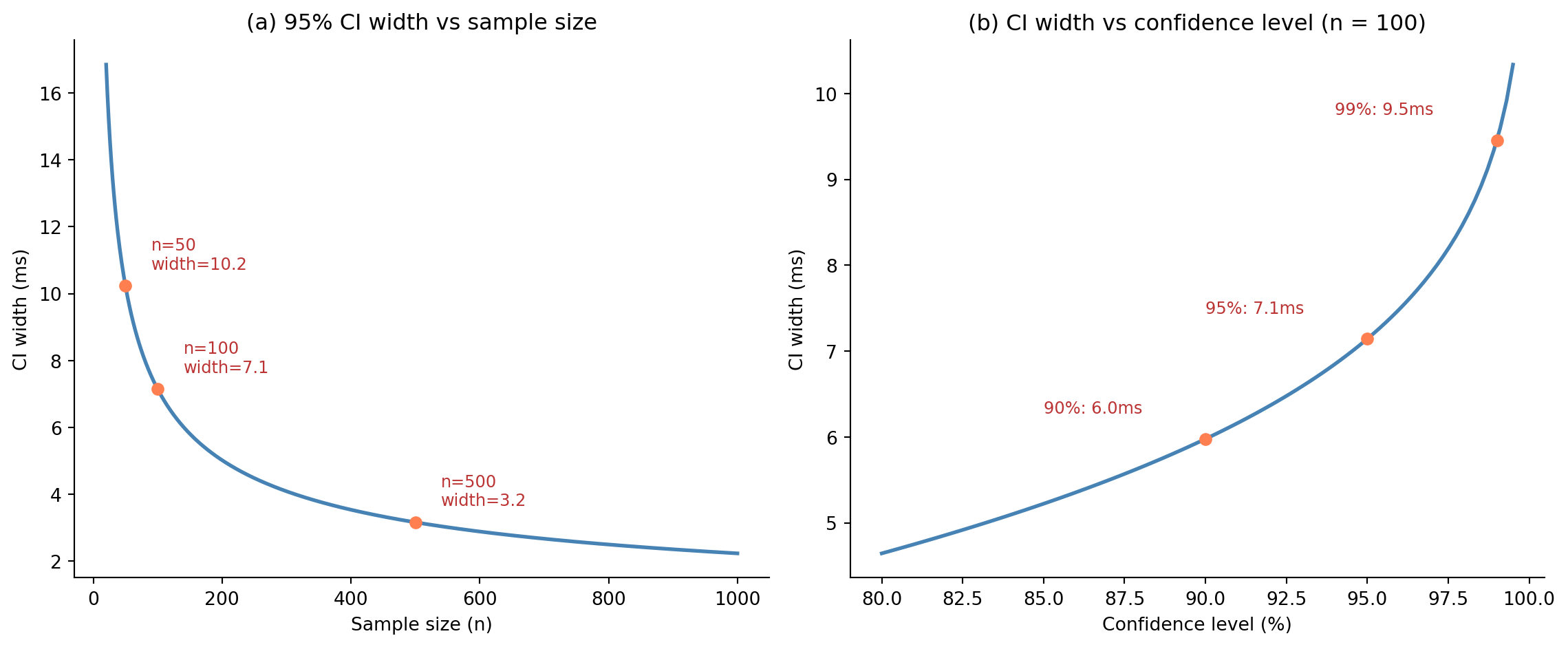
The width of a confidence interval is $2 \times t^* \times \text{standard error}$, so three factors control it. First, **sample size** ($n$): more data shrinks the SE, narrowing the interval; this is the $1/\sqrt{n}$ relationship from @sec-standard-error. Second, **variability** ($s$): noisier data means a larger SE and a wider interval. Third, the **confidence level**: higher confidence (99% vs 95%) requires a larger critical value, widening the interval. @fig-ci-width illustrates both effects: panel (a) shows how CI width shrinks with sample size, and panel (b) shows how it grows with confidence level. There's a fundamental trade-off between confidence level and interval width: you can be *more confident* that you've captured the true value, but only at the cost of a *less precise* statement about where it is. A 99.9% CI is almost guaranteed to contain the truth, but it may be so wide that it tells you nothing useful.
```{python}
#| label: fig-ci-width
#| echo: true
#| fig-cap: "CI width shrinks as sample size grows (panel a), following the √n law. Higher confidence levels require wider intervals (panel b) — the price of greater certainty."
#| fig-alt: "Two-panel line chart. Panel a shows CI width declining steeply from approximately 17ms at n=20 to about 2.2ms at n=1000, with labelled points at n=50 (10.2ms), n=100 (7.1ms), and n=500 (3.2ms). Panel b shows width increasing from about 4.7ms at 80% confidence to approximately 10.4ms at 99.5%, with labelled points at 90% (6.0ms), 95% (7.1ms), and 99% (9.5ms)."
sample_std = 18.0

# Panel (a): CI width vs sample size
fig, (ax1, ax2) = plt.subplots(1, 2, figsize=(12, 5))
fig.patch.set_alpha(0)
ax1.patch.set_alpha(0)
ax2.patch.set_alpha(0)

n_range = np.arange(20, 1001)
widths = 2 * stats.t.ppf(0.975, df=n_range - 1) * sample_std / np.sqrt(n_range)

ax1.plot(n_range, widths, '#0072B2', linewidth=2)
ax1.set_xlabel('Sample size (n)')
ax1.set_ylabel('CI width (ms)')
ax1.set_title('(a) 95% CI width vs sample size')
ax1.spines[['top', 'right']].set_visible(False)

# Mark key points
for n_mark in [50, 100, 500]:
    w = 2 * stats.t.ppf(0.975, df=n_mark - 1) * sample_std / np.sqrt(n_mark)
    ax1.plot(n_mark, w, 'o', color='#E69F00', markersize=6, zorder=5)
    ax1.annotate(f'n={n_mark}\nwidth={w:.1f}',
                 xy=(n_mark, w), xytext=(n_mark + 40, w + 0.5),
                 fontsize=9, color='#333')

# Panel (b): CI width vs confidence level
conf_levels = np.linspace(0.80, 0.995, 100)
n_fixed = 100
widths_conf = [2 * stats.t.ppf((1 + cl) / 2, df=n_fixed - 1)
               * sample_std / np.sqrt(n_fixed) for cl in conf_levels]

ax2.plot(conf_levels * 100, widths_conf, '#0072B2', linewidth=2)
ax2.set_xlabel('Confidence level (%)')
ax2.set_ylabel('CI width (ms)')
ax2.set_title(f'(b) CI width vs confidence level (n = {n_fixed})')
ax2.spines[['top', 'right']].set_visible(False)

for cl in [0.90, 0.95, 0.99]:
    w = 2 * stats.t.ppf((1 + cl) / 2, df=n_fixed - 1) * sample_std / np.sqrt(n_fixed)
    ax2.plot(cl * 100, w, 'o', color='#E69F00', markersize=6, zorder=5)
    ax2.annotate(f'{cl:.0%}: {w:.1f}ms',
                 xy=(cl * 100, w), xytext=(cl * 100 - 5, w + 0.3),
                 fontsize=9, color='#333')

plt.tight_layout()
plt.show()
```
::: {.callout-tip}
## Author's Note
The $\sqrt{n}$ law has a sting in its tail. To halve a confidence interval you need *four times* as much data. To make it ten times narrower you need a hundred times more. This is one of the few places where the engineering instinct of "just throw more capacity at it" actively misleads. The first thousand observations buy you a lot of precision; each additional batch buys proportionally less — quadrupling from 1,000 to 4,000 only halves the width again. Past a certain point, more data is the most expensive way to narrow your uncertainty: refining the measurement, reducing the source variability, or asking a less ambitious question are all cheaper. When a CI is too wide to act on, the right reaction isn't always "collect more"; sometimes it's "rephrase the question."
:::
## The bootstrap: CIs without distributional assumptions {#sec-bootstrap}
The t-interval we've been using assumes the sampling distribution is approximately Normal, which the CLT guarantees for large $n$. But what about small samples, skewed data, or statistics other than the mean (like the median or a percentile)?
The **bootstrap** [@efron1979] sidesteps the normality assumption entirely. It still assumes observations are independent and representative of the population. It relaxes the *distributional* assumption, not the *sampling* one. Since the sampling distribution describes what happens if you drew many samples from the population, and your sample is the best available stand-in for the population, just resample *from your sample*, with replacement (each observation can be selected more than once), and see how the statistic varies.
```{python}
#| label: bootstrap-ci
#| echo: true
# Simulated response times — skewed data where the t-interval may struggle
rng = np.random.default_rng(42)
# Exponential distribution: scale = mean = 50ms; naturally right-skewed
response_times = rng.exponential(scale=50, size=40)

# Bootstrap: resample with replacement, compute the statistic each time
n_bootstrap = 10_000
bootstrap_means = np.array([
    # replace=True is the core of the bootstrap — sampling with replacement
    rng.choice(response_times, size=len(response_times), replace=True).mean()
    for _ in range(n_bootstrap)
])

# The "percentile method": the 95% CI is the 2.5th and 97.5th percentiles
ci_boot = np.percentile(bootstrap_means, [2.5, 97.5])

# Compare with the t-interval
x_bar = response_times.mean()
se = response_times.std(ddof=1) / np.sqrt(len(response_times))  # ddof=1: Bessel's correction
t_crit = stats.t.ppf(0.975, df=len(response_times) - 1)
ci_t = (x_bar - t_crit * se, x_bar + t_crit * se)

print(f"Sample mean: {x_bar:.1f} ms (n = {len(response_times)})")
print(f"t-interval:       ({ci_t[0]:.1f}, {ci_t[1]:.1f})")
print(f"Bootstrap (10k):  ({ci_boot[0]:.1f}, {ci_boot[1]:.1f})")
```
```{python}
#| label: fig-bootstrap
#| echo: true
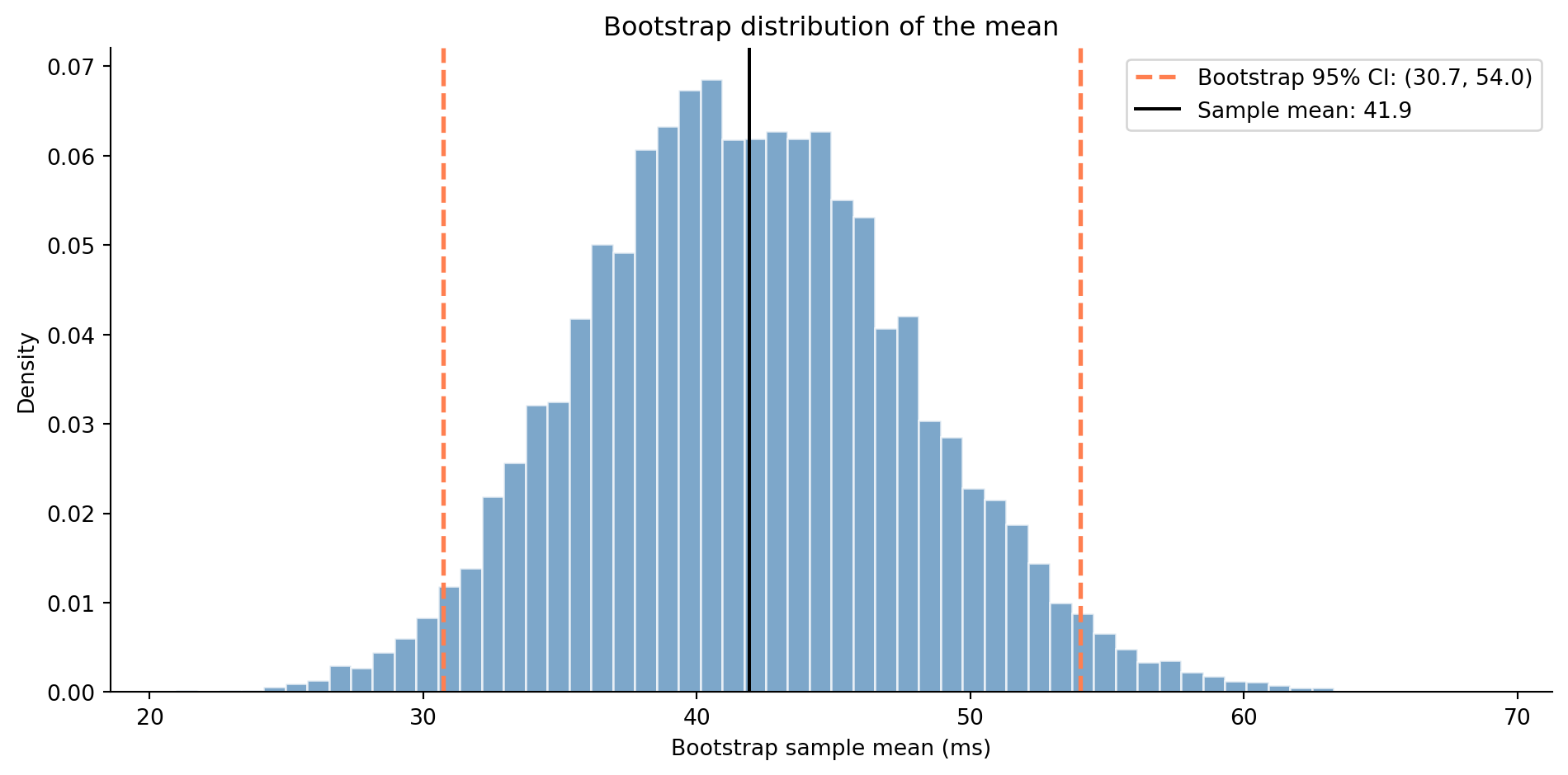
#| fig-cap: "The bootstrap distribution of the sample mean (10,000 resamples). The percentile-based CI is shown by the dashed lines. Notice the slight right skew — the bootstrap captures asymmetry that the symmetric t-interval misses."
#| fig-alt: "Histogram of 10,000 bootstrap sample means with a slight right skew. Two dashed orange vertical lines mark the 2.5th and 97.5th percentiles forming the bootstrap 95% CI, and a solid black line marks the sample mean near the centre of the distribution."
fig, ax = plt.subplots(figsize=(10, 5))
fig.patch.set_alpha(0)
ax.patch.set_alpha(0)

# density=True normalises so the y-axis shows probability density (area = 1)
ax.hist(bootstrap_means, bins=60, density=True, color='#0072B2', alpha=0.7,
        edgecolor='white')
ax.axvline(ci_boot[0], color='#E69F00', linestyle='--', linewidth=2,
           label=f'Bootstrap 95% CI: ({ci_boot[0]:.1f}, {ci_boot[1]:.1f})')
ax.axvline(ci_boot[1], color='#E69F00', linestyle='--', linewidth=2)
ax.axvline(x_bar, color='black', linewidth=1.5, label=f'Sample mean: {x_bar:.1f}')

ax.set_xlabel('Bootstrap sample mean (ms)')
ax.set_ylabel('Density')
ax.set_title('Bootstrap captures the shape of the sampling distribution')
ax.legend(loc='upper left', frameon=False)
ax.spines[['top', 'right']].set_visible(False)
plt.tight_layout()
plt.show()
```
@fig-bootstrap shows the resulting bootstrap distribution. The bootstrap has two properties that make it valuable. First, it makes **no distributional assumptions**: it works for any statistic (medians, percentiles, ratios, custom metrics) and for any sample distribution, including heavily skewed data. Second, it **captures asymmetry**: a t-interval is always symmetric around $\bar{x}$, but the bootstrap interval can be asymmetric, reflecting the actual shape of the sampling distribution. The cost is computational: instead of a single formula, you need to resample thousands of times. In practice, this is fast enough to be negligible; 10,000 is a common default, and going higher rarely changes the result meaningfully.
The percentile method shown here is the simplest bootstrap CI. More refined variants like the BCa (bias-corrected and accelerated) method correct for two issues: systematic bias in the bootstrap distribution (the "BC" part) and the way the standard error changes across the distribution, which captures skewness (the "acceleration" part). BCa maintains better coverage than the percentile method when the sample is small or the statistic is biased. `scipy.stats.bootstrap` implements several of these.
::: {.callout-note}
## Engineering Bridge
The bootstrap is **Monte Carlo simulation for statistics**. You're already comfortable with the idea: if you can't derive an analytical answer, simulate the process many times and look at the distribution of outcomes. Load testing works this way: you don't derive throughput from first principles; you hit the system with realistic traffic and measure. The bootstrap does the same thing for statistical estimates: resample, recompute, and let the distribution of results tell you the uncertainty. If you're comfortable with writing a simulation loop, you already understand the bootstrap.
:::
## Summary {#sec-confidence-intervals-summary}
1. **A confidence interval is a range of plausible values for the true parameter** — it quantifies the precision of your estimate, not just its direction.
2. **The 95% confidence level is a property of the procedure, not the result** — if you repeated the experiment many times, about 95% of the intervals would contain the true value. Any specific interval either contains it or doesn't.
3. **CIs and hypothesis tests are dual** — rejecting $H_0$ at $\alpha = 0.05$ is equivalent to the hypothesised value falling outside the 95% CI. But the CI gives you more: it tells you *where* the true value plausibly lies, not just whether to reject.
4. **Three things control CI width: sample size, variability, and confidence level.** Bigger samples and lower confidence levels give narrower intervals. The $\sqrt{n}$ law means quadrupling your data halves the width.
5. **The bootstrap provides CIs without distributional assumptions** — resample from your data and use the percentiles of the resampled statistic. It works for any statistic and captures asymmetry that formula-based intervals miss.
## Exercises {#sec-confidence-intervals-exercises}
1. A load balancer reports the following response times (in ms) for 15 sampled requests: `[23, 31, 45, 27, 33, 52, 38, 29, 41, 36, 48, 25, 30, 44, 35]`. Compute a 95% confidence interval for the mean using the t-distribution (manually with `numpy`/`scipy`, then verify with `stats.t.interval`). Interpret the result: what range of true mean response times is consistent with this data?
2. Your A/B test ran for two weeks and measured conversion rates of 8.2% (control, $n = 5\text{,}000$) and 9.1% (variant, $n = 5\text{,}000$). Compute 95% CIs for each group and for the difference. Does the CI for the difference include zero? Based on the CI width, was this experiment well-powered for detecting a meaningful effect?
3. **Bootstrap vs t-interval.** Generate 30 observations from a lognormal distribution — a heavily right-skewed distribution where the logarithm of the values is normally distributed — using `rng.lognormal(mean=3, sigma=1, size=30)`. Compute both a t-based 95% CI and a bootstrap 95% CI (using 10,000 resamples) for the mean. How do they compare? Repeat with $n = 200$. At what point does the t-interval become reliable for skewed data, and why?
4. Create a simulation that demonstrates the coverage property of confidence intervals. For a known population (e.g., Normal(100, 15)), draw 1,000 samples of size $n = 50$, compute a 95% CI for each, and count how many contain the true mean. Repeat with 90% and 99% CIs. Do the actual coverage rates match the stated confidence levels?
5. **Conceptual:** A colleague reports "the 95% CI for the mean is (42, 58), so there's a 95% probability that the true mean is between 42 and 58." What's wrong with this statement? How would you explain the correct interpretation? Then consider: from a *decision-making* standpoint, does the distinction actually matter in practice? When might the incorrect interpretation lead you astray?