def generate_invoice(price: float, quantity: int, tax_rate: float) -> float:
    """Same inputs → same output. We bet our test suites on this."""
    return round(price * quantity * (1 + tax_rate), 2)

# The assertion encodes what we expect to see if nothing is wrong
assert generate_invoice(9.99, 3, 0.20) == 35.965 Hypothesis testing: the unit test of data science
5.1 Every test starts with an assumption
Every unit test you’ve ever written follows the same logic: assume the code is correct, run it, and check whether the output is consistent with that assumption. If the output contradicts the assumption, the test fails. Remember the generate_invoice function from Section 1.1:
The assertion encodes your expectation under a specific assumption, the function works correctly. When the test fails, you don’t conclude “something might be broken.” You conclude the code doesn’t behave as expected and investigate.
Hypothesis testing applies the same logic to data. You start with an assumption, typically “there is no effect” or “nothing has changed”, and ask whether the data is consistent with that assumption. If the data is sufficiently surprising under the assumption, you reject it.
The difference is that with code, the assertion is exact: 35.96 or not. With data, you’re dealing with the sampling variability we explored in Section 4.4. The output is never exactly what you expect, even when nothing is wrong. So the question becomes: how far from the expected value does the data need to be before you conclude something real is happening?
5.2 The framework: assume, measure, decide
A hypothesis test has five components. Consider a concrete case that any backend engineer will recognise.
Your SLO (service-level objective) says mean API response time should be 50ms. A recent sample of 100 requests shows a mean of 54.2ms with a standard deviation of 18ms. Is the service degraded, or is this normal variation?
Step 1: State the hypotheses. The assumption you test against is the null hypothesis, \(H_0\). The claim you’re investigating is the alternative hypothesis, \(H_1\).
- \(H_0\): The true mean response time is 50ms. (\(\mu = 50\))
- \(H_1\): The true mean response time is not 50ms. (\(\mu \neq 50\))
The null hypothesis isn’t something you believe; it’s something you test against. Just as a unit test doesn’t prove correctness (it only fails to find a bug), a hypothesis test doesn’t prove \(H_0\). It only asks whether the data provides enough evidence to reject it.
Step 2: Compute the test statistic. You need a single number that captures how far the observed result is from what \(H_0\) predicts. For comparing a sample mean to an expected value, the standard choice is the t-statistic:
\[ t = \frac{\bar{x} - \mu_0}{s / \sqrt{n}} \]
where \(\bar{x}\) is the sample mean, \(\mu_0\) is the value expected under \(H_0\) (the subscript 0 is a convention meaning “under the null”), \(s\) is the sample standard deviation, and \(n\) is the sample size. This should look familiar from Section 4.6: the denominator \(s / \sqrt{n}\) is the standard error. The t-statistic measures how many standard errors the sample mean is from the hypothesised value.
from scipy import stats

# Observed summary statistics
sample_mean = 54.2
hypothesised_mean = 50.0
sample_std = 18.0
n = 100

# How many standard errors from the hypothesised mean?
se = sample_std / np.sqrt(n)
t_stat = (sample_mean - hypothesised_mean) / se

print(f"Sample mean:    {sample_mean} ms")
print(f"Expected (H₀):  {hypothesised_mean} ms")
print(f"Standard error: {se:.2f} ms")
print(f"t-statistic:    {t_stat:.2f}")
Sample mean: 54.2 ms
Expected (H₀): 50.0 ms
Standard error: 1.80 ms
t-statistic: 2.33A t-statistic of 2.33 means the sample mean is 2.33 standard errors above what \(H_0\) predicts. If \(H_0\) were true, the Central Limit Theorem (CLT; see Section 4.5) tells us the sampling distribution of the mean is approximately Normal, but because we estimate \(\sigma\) with the sample standard deviation \(s\), the test statistic follows a t-distribution rather than a standard Normal.
Think of it as a Normal distribution with slightly fatter tails, more probability mass in the extremes, because dividing by \(s\) (a random variable estimated from the data) rather than \(\sigma\) (a fixed constant) introduces extra variability. With \(n = 10\), your estimate of \(s\) could easily be off by around a quarter (its relative standard deviation is roughly \(1/\sqrt{2(n-1)} \approx 24\%\)), so you need to account for the fact that your ruler itself is imprecise. With \(n = 100\) (so degrees of freedom \(= 99\)), the difference is negligible, and the distinction fades further as \(n\) grows.
The t-test assumes the underlying data is approximately normally distributed, or that \(n\) is large enough for the CLT to make the sampling distribution of the mean approximately Normal; the conventional rule of thumb is \(n \geq 30\), though heavily skewed distributions may require more. When that assumption doesn’t hold and your sample is small, non-parametric tests (covered in Section 5.7) offer an alternative.
Step 3: Compute the p-value. The p-value is the probability of observing a test statistic at least as extreme as the one you got, assuming \(H_0\) is true. In other words: if there really were no change, how often would random sampling alone produce a result this far from 50ms?
# sf = "survival function" = 1 - CDF = P(T > t) — a scipy convention
# df = degrees of freedom = n - 1 (we lose one because s uses x̄ to estimate σ)
# 2× because this is a two-sided test: we'd be equally surprised by 45.8ms as by 54.2ms
p_value = 2 * stats.t.sf(abs(t_stat), df=n - 1)

print(f"p-value: {p_value:.4f}")
print(f"\nIf the true mean were 50ms, there's a {p_value:.1%} chance")
print(f"of seeing a sample mean this far from 50.")
p-value: 0.0217
If the true mean were 50ms, there's a 2.2% chance
of seeing a sample mean this far from 50.We use a two-sided test here because we’d investigate whether response times went up or down from 50ms. If you only cared about increases (a one-sided test), you’d drop the factor of 2 and the p-value would be half as large. Most scipy test functions default to two-sided; the alternative parameter controls this. When in doubt, two-sided is the safer choice: it’s harder to reach significance, but you won’t miss effects in the unexpected direction.
Step 4: Set the significance level. The significance level \(\alpha\) is your threshold, the false positive rate you’re willing to tolerate. The conventional choice is \(\alpha = 0.05\): you’ll reject \(H_0\) if the p-value falls below 5%. Crucially, you should choose \(\alpha\) before looking at the data; choosing it after is like writing your assertion after seeing the output.
Step 5: Decide. Compare the p-value to \(\alpha\) and draw your conclusion.
alpha = 0.05

if p_value < alpha:
    print(f"p = {p_value:.4f} < α = {alpha}")
    print('Reject H₀: evidence suggests response times have shifted from 50ms.')
else:
    print(f"p = {p_value:.4f} ≥ α = {alpha}")
    print('Fail to reject H₀: insufficient evidence of a shift.')
p = 0.0217 < α = 0.05
Reject H₀: evidence suggests response times have shifted from 50ms.Notice the phrasing: “fail to reject,” not “accept.” You don’t “accept” \(H_0\); absence of evidence is not evidence of absence. The test might simply lack the power to detect a real shift. We’ll quantify this precisely in Section 5.5.
This approach (reasoning about what would happen across many hypothetical repetitions of the experiment) is the hallmark of frequentist inference, the statistical paradigm this chapter works within. We’ll contrast it with the Bayesian alternative in Bayesian inference: updating beliefs with evidence.
Let’s verify our manual calculation against scipy’s built-in t-test. We’ll use stats.ttest_1samp on actual sample data; note that the function needs the raw observations, not summary statistics.
# Draw a sample, then rescale it to hit our summary statistics *exactly*
# (x̄ = 54.2, s = 18.0). A raw random draw won't match those figures, and a
# sample whose mean and std both differ would only agree with the manual
# t-statistic by coincidence — two errors cancelling. Standardising makes this
# a genuine cross-check of the arithmetic.
rng = np.random.default_rng(42)
raw = rng.normal(loc=54.2, scale=18.0, size=100)
sample_data = (raw - raw.mean()) / raw.std(ddof=1) * 18.0 + 54.2  # ddof=1: n-1

# scipy's one-sample t-test against the SLO target
# popmean: the H₀ value we're testing against, not the actual population mean
t_scipy, p_scipy = stats.ttest_1samp(sample_data, popmean=50.0)
print(f"scipy:  t = {t_scipy:.2f}, p = {p_scipy:.4f}")
print(f"manual: t = {t_stat:.2f}, p = {p_value:.4f}")
print(f"\nThe two agree exactly: by construction the sample has "
      f"x̄ = {sample_data.mean():.1f} and s = {sample_data.std(ddof=1):.1f}, "
      f"the same summary statistics we used by hand.")
scipy: t = 2.33, p = 0.0217
manual: t = 2.33, p = 0.0217
The two agree exactly: by construction the sample has x̄ = 54.2 and s = 18.0, the same summary statistics we used by hand.
NoteEngineering Bridge
The logic here is identical to how you reason about flaky tests. If a test fails once out of a hundred runs, you might chalk it up to a race condition. If it fails twenty times out of a hundred, something is genuinely broken. The p-value formalises this intuition: it tells you how unlikely your observation is under the “nothing is wrong” assumption. The significance level \(\alpha\) is your tolerance threshold, how much flakiness you’re willing to accept before you investigate. Setting \(\alpha = 0.05\) is like saying “if this would happen by chance less than 5% of the time, I’m treating it as a real issue.”
5.3 Resolving the A/B test
In Section 4.7, we left a question hanging. Your checkout A/B test showed a 12.0% conversion rate for the control (\(n = 1\text{,}000\)) and 13.5% for the variant (\(n = 1\text{,}000\)). The sampling distributions overlapped substantially, and the z-score was about 1.0. Now we can answer: is the difference real?
For comparing two proportions, the test statistic is:
\[ z = \frac{\hat{p}_1 - \hat{p}_2}{\sqrt{\hat{p}(1 - \hat{p})\left(\frac{1}{n_1} + \frac{1}{n_2}\right)}} \]
where \(\hat{p}_1\) and \(\hat{p}_2\) are the observed conversion rates (the hat means “estimated from data,” as in Section 4.6), and \(\hat{p}\) is the pooled proportion, the total number of conversions divided by the total number of users across both groups. Why pool? Under \(H_0\), both groups share the same underlying rate, so combining them gives the best estimate of that shared rate and therefore the most accurate standard error for the difference.
# A/B test data from the probability chapter
n_control, n_variant = 1000, 1000
p_control, p_variant = 0.120, 0.135

# Pooled proportion under H0
# (p_control * n_control is the conversion count, so this is total conversions
#  divided by total users — exactly the pooled rate described above)
p_pooled = (p_control * n_control + p_variant * n_variant) / (n_control + n_variant)

# Standard error of the difference under H0
se_diff = np.sqrt(p_pooled * (1 - p_pooled) * (1/n_control + 1/n_variant))

# z-statistic
z = (p_variant - p_control) / se_diff

# Normal (not t) because the two-proportion z-test is a large-sample approximation.
# Unlike the t-statistic, there is no exact closed-form null distribution for this
# test statistic — the Normal approximation holds when np and n(1-p) are both >> 5
# (here both are ~120 and ~880, so the approximation is excellent).
# For small n, Fisher's exact test is the appropriate alternative.
p_value_ab = 2 * stats.norm.sf(abs(z))  # sf = survival function (see earlier)

print(f"Control:     {p_control:.1%} (n = {n_control})")
print(f"Variant:     {p_variant:.1%} (n = {n_variant})")
print(f"Pooled rate: {p_pooled:.1%}")
print(f"SE (diff):   {se_diff:.4f}")
print(f"z-statistic: {z:.2f}")
print(f"p-value:     {p_value_ab:.4f}")

if p_value_ab < 0.05:
    print('\nReject H₀: the difference is statistically significant.')
else:
    print('\nFail to reject H₀: insufficient evidence of a real difference.')
Control: 12.0% (n = 1000)
Variant: 13.5% (n = 1000)
Pooled rate: 12.8%
SE (diff): 0.0149
z-statistic: 1.01
p-value: 0.3146
Fail to reject H₀: insufficient evidence of a real difference.The p-value is well above 0.05. The 1.5 percentage point difference could be real, but the data doesn’t provide strong enough evidence to distinguish it from sampling noise at this sample size. Note that this test assumes independence both between groups (no user appears in both) and within groups (each conversion is an independent event). In practice, device sharing or social contagion can violate this, a consideration we’ll revisit in A/B testing: deploying experiments.
x = np.linspace(-4, 4, 300)
fig, ax = plt.subplots(figsize=(10, 5))
fig.patch.set_alpha(0)
ax.patch.set_alpha(0)

# Null distribution
ax.plot(x, stats.norm.pdf(x), '#0072B2', linewidth=2, label='Distribution under H₀')

# Rejection regions
alpha = 0.05
z_crit = stats.norm.ppf(1 - alpha / 2)  # ppf = inverse CDF (quantile function)
x_left = x[x <= -z_crit]
x_right = x[x >= z_crit]
ax.fill_between(x_left, stats.norm.pdf(x_left), alpha=0.5, color='#E69F00',
                label=f'Rejection region (α = {alpha})')
ax.fill_between(x_right, stats.norm.pdf(x_right), alpha=0.5, color='#E69F00')

# Observed z
ax.axvline(z, color='black', linewidth=2, linestyle='--',
           label=f'Observed z = {z:.2f}')

# Critical values — annotate both sides
ax.axvline(-z_crit, color='#E69F00', linewidth=1, linestyle=':')
ax.axvline(z_crit, color='#E69F00', linewidth=1, linestyle=':')
ax.annotate(f'z = −{z_crit:.2f}', xy=(-z_crit - 0.1, 0.07), fontsize=10,
            color='black', ha='right')
ax.annotate(f'z = +{z_crit:.2f}', xy=(z_crit + 0.1, 0.07), fontsize=10,
            color='black', ha='left')

ax.set_xlabel('z-statistic')
ax.set_ylabel('Density')
ax.set_title(f'Observed z = {z:.2f} — not extreme enough to reject H₀ at α = 0.05')
ax.legend(loc='upper right')
for spine in ['top', 'right']:
    ax.spines[spine].set_visible(False)
plt.tight_layout()
plt.show()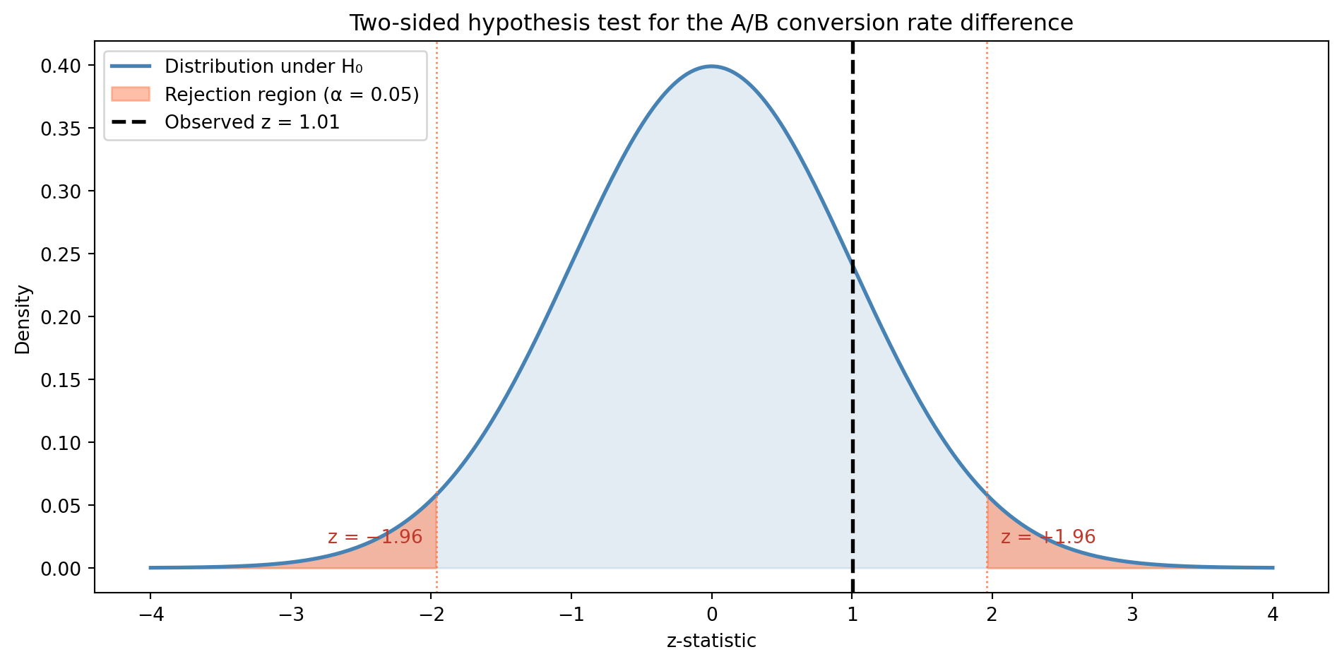
This doesn’t mean the variant is definitely no better; it means we don’t have enough data to be confident. We’ll return to this distinction in Confidence intervals: error bounds for estimates, where we’ll quantify the range of plausible true differences. And in A/B testing: deploying experiments, we’ll learn how to design tests with adequate power.
5.4 Two ways to be wrong
Every decision has two ways to go wrong. A hypothesis test is no different.
A Type I error (false positive) occurs when you reject \(H_0\) even though it’s true: you conclude there’s an effect when there isn’t one. The significance level \(\alpha\) directly controls this: setting \(\alpha = 0.05\) means you accept a 5% chance of a false positive.
A Type II error (false negative) occurs when you fail to reject \(H_0\) even though it’s false: you miss a real effect. The probability of a Type II error is denoted \(\beta\).
| Decision | \(H_0\) is true (no effect) | \(H_0\) is false (real effect) |
|---|---|---|
| Reject \(H_0\) | Type I error (\(\alpha\)) | Correct detection |
| Fail to reject \(H_0\) | Correct | Type II error (\(\beta\)) |
The two error types trade off against each other. Lower your \(\alpha\) (be more cautious about false positives) and you increase \(\beta\) (miss more real effects). Raise \(\alpha\) (be more willing to act on weak evidence) and you catch more real effects but also generate more false alarms.
NoteEngineering Bridge
This is the precision–recall trade-off under a different name. In a classification system, precision measures how many of your positive predictions are correct (analogous to controlling false positives via \(\alpha\)). Recall measures how many actual positives you catch (analogous to \(1 - \beta\), the power, how often you detect real effects). You can’t maximise both simultaneously: tightening your detection threshold reduces false alarms but also misses more real events. The optimal balance depends on the cost of each error type, and in hypothesis testing, just as in alerting, those costs are rarely symmetric.
5.5 Power: will you detect what matters?
Statistical power is the probability of correctly rejecting \(H_0\) when it’s actually false, the probability of detecting a real effect. Power equals \(1 - \beta\).
Power depends on three things. First, the effect size (how large the real difference is), because bigger effects are easier to detect. Second, the sample size, because more data gives you more precision (lower standard error), making it easier to distinguish signal from noise. Third, the significance level \(\alpha\), because a stricter threshold makes it harder to reject \(H_0\), reducing power.
A common target is 80% power: you want at least an 80% chance of detecting the effect if it exists. Power analysis lets you calculate the sample size needed to achieve this, given the effect size you care about.
from statsmodels.stats.power import NormalIndPower

# NormalIndPower handles power analysis for two independent groups using the
# Normal approximation — suitable for proportion comparisons at reasonable n.
# Its solve_power method takes any three of {effect_size, nobs1, alpha, power}
# and solves for the fourth.
power_analysis = NormalIndPower()

# How many users per group to detect a 2 percentage point (pp) difference
# (12% → 14%) with 80% power at α = 0.05?

# To use NormalIndPower, we need a standardised effect size that accounts for
# the fact that proportions near 0% or 100% have less variability than those
# near 50%. Cohen's h does this via an arcsine transformation:
#   h = 2 * (arcsin(√p₂) - arcsin(√p₁))
# You don't need to memorise the formula — just know that it puts proportion
# differences on a common scale so the power calculator can work with them.
# (For continuous data, the equivalent is Cohen's d — the difference in means
# divided by the pooled standard deviation.)
baseline = 0.12
target = 0.14
cohens_h = 2 * (np.arcsin(np.sqrt(target)) - np.arcsin(np.sqrt(baseline)))

n_needed = power_analysis.solve_power(
    effect_size=cohens_h,
    alpha=0.05,
    power=0.80,
    alternative='two-sided'
)

print(f"Effect size (Cohen's h): {cohens_h:.4f}")
print(f"Required n per group:    {np.ceil(n_needed):.0f}")
print(f"\nTo detect a 2pp lift (12% → 14%) with 80% power,")
print(f"you need ~{np.ceil(n_needed):.0f} users per group.")
Effect size (Cohen's h): 0.0595
Required n per group: 4433
To detect a 2pp lift (12% → 14%) with 80% power,
you need ~4433 users per group.This explains why our A/B test in Section 5.3 failed to reach significance. With 1,000 users per group, the test was underpowered: it didn’t have enough data to reliably detect a 1.5 percentage point (pp) difference.
# Okabe-Ito colourblind-safe palette
colours = ['#0072B2', '#E69F00', '#009E73', '#CC79A7']
markers = ['o', 's', '^', 'D']
linestyles = ['-', '--', '-.', ':']

fig, ax = plt.subplots(figsize=(10, 5))
fig.patch.set_alpha(0)
ax.patch.set_alpha(0)

baseline_rate = 0.12
pp_diffs = np.linspace(0.005, 0.06, 200)

for i, n_per_group in enumerate([500, 1000, 2500, 5000]):
    # statsmodels' power() doesn't broadcast, so we loop over effect sizes
    powers = [
        power_analysis.power(
            effect_size=2 * (np.arcsin(np.sqrt(baseline_rate + diff))
                             - np.arcsin(np.sqrt(baseline_rate))),
            nobs1=n_per_group, alpha=0.05, alternative='two-sided'
        )
        for diff in pp_diffs
    ]
    ax.plot(pp_diffs * 100, powers, linewidth=2, linestyle=linestyles[i],
            color=colours[i], marker=markers[i], markevery=25, markersize=6,
            label=f'n = {n_per_group:,}')

ax.axhline(y=0.80, color='grey', linestyle='--', alpha=0.7, label='80% power')
ax.axvline(x=1.5, color='grey', linestyle=':', alpha=0.6)
ax.annotate('Our A/B test\n(1.5pp diff)', xy=(1.5, 0.12), fontsize=10,
            color='#555555', ha='center', va='bottom')

ax.set_xlabel('Conversion rate difference (percentage points)')
ax.set_ylabel('Power (probability of detecting the difference)')
ax.set_title('Power curves: how much data do you need?')
ax.legend()
ax.set_ylim(0, 1.05)
ax.yaxis.grid(True, linestyle=':', alpha=0.4, color='grey')
ax.set_axisbelow(True)
for spine in ['top', 'right']:
    ax.spines[spine].set_visible(False)
plt.tight_layout()
plt.show()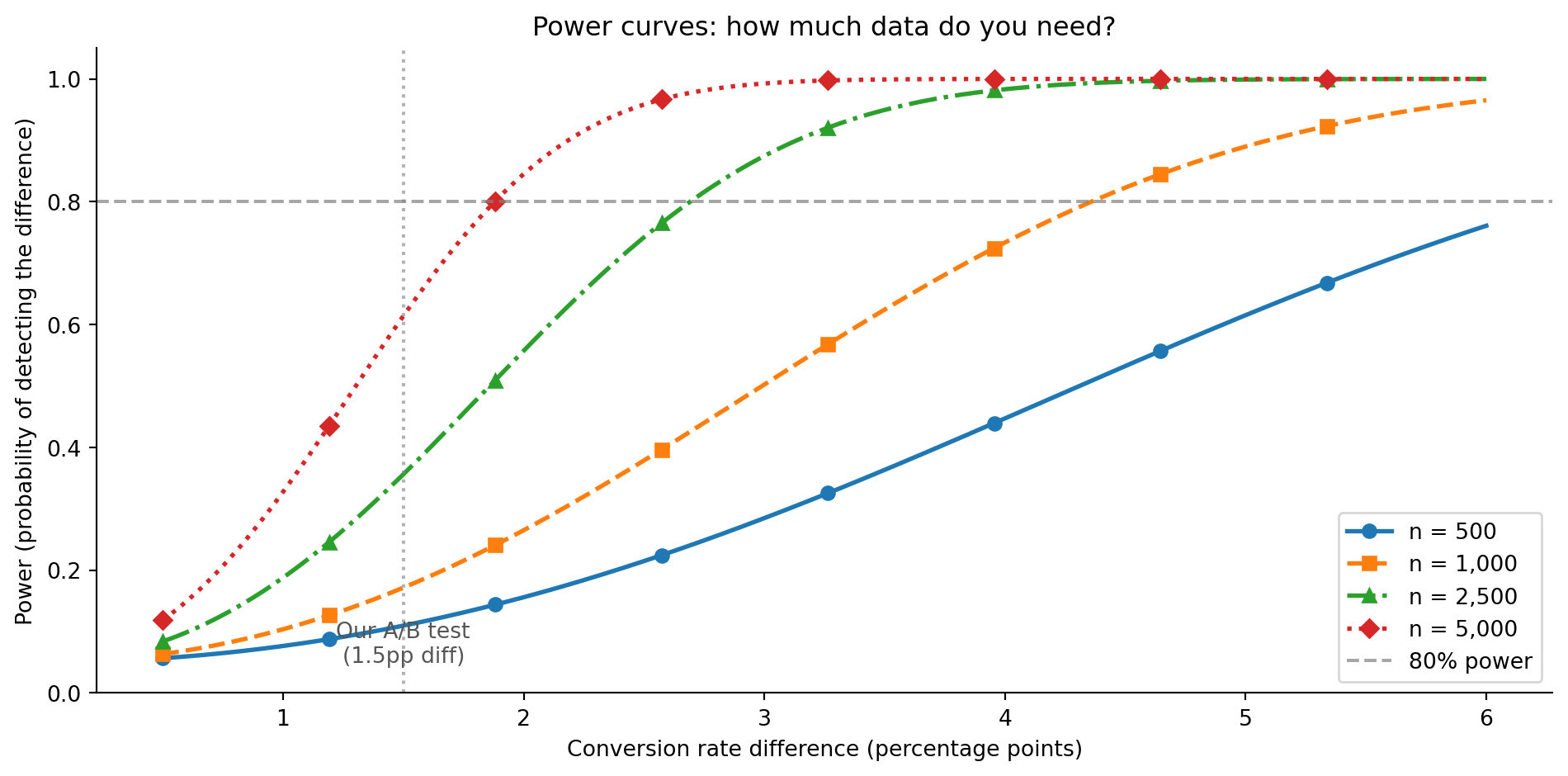
TipAuthor’s Note
Power analysis challenges a deep engineering instinct: work with whatever data you have and make the best decision you can. But that’s like running a test suite with arbitrary coverage and trusting the result. Deciding your sample size before the experiment is essential. It’s the difference between a test that can actually answer your question and one that’s doomed to be inconclusive. You wouldn’t ship a test suite with 10% coverage and conclude “no bugs” when everything passes. An underpowered hypothesis test is the statistical equivalent of low test coverage: it’s not that the bugs aren’t there, it’s that you’re not looking hard enough.
5.6 What the p-value is not
The p-value is one of the most misunderstood quantities in statistics. Before we go further, let’s be explicit about three things it does not mean.
It is not the probability that \(H_0\) is true. A p-value of 0.03 does not mean “there’s a 3% chance of no effect.” It means “if there were no effect, there’s a 3% chance of seeing data this extreme.” The distinction is between \(P(\text{data} \mid H_0)\), the probability of the data given \(H_0\), and \(P(H_0 \mid \text{data})\), the probability of \(H_0\) given the data. The frequentist approach we’ve been using (computing p-values, setting \(\alpha\) thresholds, reasoning about “what would happen in repeated samples”) only gives us \(P(\text{data} \mid H_0)\). To flip the conditional and compute \(P(H_0 \mid \text{data})\) directly, you need Bayes’ theorem and a prior, which is exactly what Bayesian inference: updating beliefs with evidence addresses.
It is not a measure of effect size. A tiny, meaningless difference can be “statistically significant” with enough data. If you test 10 million users, you can detect a 0.01 percentage point conversion difference, real but not worth acting on. Statistical significance and practical significance are different things. Always report the effect size alongside the p-value.
It is not reliable under repeated testing. If you test 20 hypotheses at \(\alpha = 0.05\), you’d expect one false positive by chance alone, even when none of the effects are real. Every time you “just check one more metric” or “slice the data one more way,” you inflate your false positive rate. This is the multiple testing problem.
rng = np.random.default_rng(42)

# Simulate 20 A/B tests where there is NO real effect
n_tests = 20
n_per_group = 1000
false_positives = 0

for i in range(n_tests):
    # Both groups drawn from the same distribution — no real difference
    control = rng.binomial(1, 0.10, size=n_per_group)
    variant = rng.binomial(1, 0.10, size=n_per_group)

    # A t-test on 0/1 data works here because at n = 1,000 the CLT makes the
    # sampling distribution of the mean approximately Normal
    _, p = stats.ttest_ind(control, variant)

    if p < 0.05:
        false_positives += 1
        print(f"  Test {i + 1:>2}: p = {p:.4f} — 'significant' (false positive)")

print(f"\n{false_positives} false positives out of {n_tests} tests (no real effects)")
print(f"Expected by chance: {n_tests * 0.05:.0f}")
Test 6: p = 0.0319 — 'significant' (false positive)
1 false positives out of 20 tests (no real effects)
Expected by chance: 1The fix is to adjust \(\alpha\) when testing multiple hypotheses. The simplest approach is the Bonferroni correction: divide \(\alpha\) by the number of tests \(k\). If each test uses a threshold of \(\alpha/k\), the overall chance of at least one false positive is at most \(\alpha\), regardless of whether the tests are independent. This makes Bonferroni widely applicable but conservative; it controls false positives at the cost of reduced power. More sophisticated methods like false discovery rate (FDR) control, most commonly the Benjamini–Hochberg procedure, allow more detections by controlling the expected proportion of false positives among rejected hypotheses, rather than the probability of any false positive. We’ll return to both in A/B testing: deploying experiments, where multiple comparisons are a constant practical concern.
TipAuthor’s Note
The natural misreading of \(p = 0.03\) as “3% chance the null is true” is almost irresistible because it feels so clean. What makes it wrong is easier to see with a different framing: a stack trace tells you \(P(\text{this trace} \mid \text{this bug})\), not \(P(\text{this bug} \mid \text{this trace})\). A NullPointerException is consistent with a null reference bug, but it could also come from a dozen other causes. You’ve seen that exception dozens of times and you almost always know the cause, but that’s because you’ve already built up context about which bugs are likely. That implicit prior is exactly what the Bayesian approach formalises, and why the p-value on its own can’t tell you what you most want to know.
5.7 Choosing the right test
We’ve used two tests so far: the one-sample t-test and the two-proportion z-test. In practice, the choice of test depends on what you’re comparing and the type of data you have.
| Scenario | Test | Function |
|---|---|---|
| One sample mean vs known value | One-sample t-test | stats.ttest_1samp |
| Two independent sample means | Two-sample t-test | stats.ttest_ind |
| Two paired sample means | Paired t-test | stats.ttest_rel |
| Two proportions | z-test for proportions | Manual (as above) |
| More than two group means | One-way ANOVA | stats.f_oneway |
| Non-normal data, small \(n\) | Mann–Whitney U test | stats.mannwhitneyu |
A few notes on the table. Use a paired test when the two measurements come from the same subjects (e.g., response times before and after a code change on the same endpoints); ttest_rel stands for “related samples.” ANOVA (Analysis of Variance) extends the t-test to three or more groups, testing whether any group mean differs from the others; it tells you that at least one group is different but not which pairs differ (you need post-hoc tests like Tukey’s HSD, Honest Significant Difference, for that). ANOVA avoids the multiple-testing problem that would arise from running separate t-tests for every pair.
The t-test assumes the data is approximately normally distributed, or that \(n\) is large enough for the CLT (see Section 4.5) to make the sampling distribution approximately Normal. When that assumption doesn’t hold and your sample is small, non-parametric tests make fewer assumptions about the underlying distribution. Mann–Whitney, for example, converts values to ranks: it sorts all observations from both groups together and works with their ordinal positions rather than the raw measurements, which makes it insensitive to outliers and skew, at the cost of somewhat lower power when normality does hold. Strictly, it tests whether values from one group tend to be consistently larger than values from the other (known as stochastic ordering), rather than testing a difference in means directly.
One practical tip: ttest_ind accepts an equal_var parameter. The default (True) assumes both groups have the same variance; setting equal_var=False uses Welch’s t-test, which doesn’t require this assumption and is generally the safer default.
Don’t agonise over the choice. For most practical purposes with \(n > 30\), the t-test is robust enough. The bigger risk isn’t choosing the wrong test — it’s misinterpreting the result.
5.8 Summary
Hypothesis testing follows the logic of unit testing — assume nothing is wrong (\(H_0\)), measure the data, and reject the assumption only if the evidence is strong enough.
The test statistic measures how far the data is from the null hypothesis, expressed in standard-error units. The p-value tells you how surprising that distance is under \(H_0\).
The p-value is not the probability that \(H_0\) is true — it’s the probability of seeing data this extreme if \(H_0\) were true. Statistical significance and practical significance are different things.
Type I and Type II errors trade off like precision and recall — reducing false positives (lower \(\alpha\)) increases false negatives (lower power). Power analysis tells you how much data you need to detect effects that matter.
Always decide your sample size before the experiment — running underpowered tests is like shipping with low test coverage. A non-significant result doesn’t mean “no effect”; it might mean “not enough data.”
5.9 Exercises
Your monitoring system reports that the historical mean response time for an API endpoint is 120ms. You collect a sample of 200 recent requests and find a mean of 127ms with a standard deviation of 45ms. Using a one-sample t-test at \(\alpha = 0.05\), is there evidence that response times have changed? Compute the t-statistic and p-value manually, then verify with
scipy.stats.ttest_1samp(generate sample data consistent with the summary statistics usingrng.normal(127, 45, 200)).Two versions of a search algorithm are tested on query speed. Version A (\(n = 150\)) has a mean of 340ms with a standard deviation of 80ms. Version B (\(n = 150\)) has a mean of 315ms with a standard deviation of 75ms. Use
scipy.stats.ttest_indto test whether the difference is significant. Then compute Cohen’s \(d\) (\(d = |\bar{x}_1 - \bar{x}_2| / s_{\text{pooled}}\), where \(s_{\text{pooled}} = \sqrt{(s_1^2 + s_2^2) / 2}\) — this simplified form assumes equal group sizes) to assess practical significance. Is the difference large enough to justify switching algorithms?Using
statsmodels.stats.power.NormalIndPower, create a table showing the required sample size per group to detect conversion rate differences of 0.5, 1.0, 2.0, and 5.0 percentage points from a 10% baseline, all at 80% power with \(\alpha = 0.05\). What does the relationship between effect size and required sample size tell you about planning A/B tests?Simulate the multiple testing problem: run 100 independent two-sample t-tests where \(H_0\) is true for all of them (both groups drawn from the same Normal distribution). Count how many produce \(p < 0.05\). Now apply the Bonferroni correction (use \(\alpha / 100 = 0.0005\) as your threshold). How many false positives remain? What is the trade-off?
Conceptual: A colleague runs an A/B test with 50 users per group and finds \(p = 0.25\). They conclude: “There’s no difference between the variants.” What is wrong with this conclusion? What would you advise them to do differently? (Hint: think about power.)
Conceptual: This chapter frames a hypothesis test as the unit test of data science. Where does that analogy break down? Address at least three differences: what happens when you re-run each one, what a “pass” (a non-significant result) actually licenses you to conclude, and whether the outcome is deterministic given the same code and data.